Data Structures and Algorithms

---

Timeline

Timeline

2025-09-28

add Introduction

2025-10-18

add Linear List, Stack, Queue, Array, String

2025-10-20

add Tree, Graph

2025-11-09

add DSU (Disjoint Set Union)

2026-03-22

add Algorithm

This article introduces the basic concepts and core content of data structures and algorithms. It first elaborates on the logical structure and storage structure of data, including linear structures, tree structures, graph structures, and four storage methods: sequential, linked, indexed, and hashed. It then explains the five basic characteristics of algorithms (finiteness, definiteness, feasibility, input, and output) and the measurement methods of algorithm efficiency, focusing on the representation of time complexity and common asymptotic complexity. In the data structure section, it discusses in detail the sequential representation and linked representation of linear lists (singly linked list, doubly linked list, circular linked list, static linked list), and provides implementation ideas in languages such as C, C++, and Rust, as well as time complexity analysis of basic operations. The article also introduces the definition and characteristics of stacks (last in, first out), the Catalan number formula for stack pop sequences, and the sequential storage, shared stack, and linked storage structures of stacks. Overall, the content covers the fundamentals of data structures and algorithms and is suitable as an introductory reference for learning.

---

Introduction

Logical Structure of Data

The logical structure of data refers to the relationships among data elements, that is, describing data in terms of logical relations. It is independent of data storage and is independent of the computer.

• Linear Structure
  • Linear list
    • Array
    • Stack
    • Queue
• Nonlinear Structure
  • Set
  • Tree Structure
    • General Tree
    • Binary Tree
  • Graph Structure
    • Directed graph
    • Undirected graph

Storage Structure of Data

The storage structure refers to the representation of a data structure in a computer, also called the physical structure.

• Sequential Storage

Sequential storage means storing logically adjacent elements in storage units that are also adjacent in physical location;

• Linked Storage

Linked storage uses pointers that indicate the storage addresses of elements to represent the logical relationships between elements;

• Index storage

Index storage means that while storing element information, an additional index table is also established. Each item in the index table is called an index entry, and the general form of an index entry is (key, address);

• Hash storage

Hash storage is a method that directly calculates the storage address of an element based on its key, also known as hash storage.

Basic concepts of algorithms

• Finiteness

Finiteness means that an algorithm must always terminate after a finite number of steps, and each step must be completed in finite time;

• Definiteness

Definiteness means that every instruction in the algorithm must have an unambiguous meaning, and for the same input, only the same output can be obtained;

• Effectiveness

Effectiveness means that the operations described in the algorithm can all be implemented by performing already implemented basic operations a finite number of times;

• Input

Input means that an algorithm has zero or more inputs, which are taken from a specific set of objects.

• output

Output means that an algorithm has one or more outputs, which are quantities that have a specific relationship with the inputs.

Measurement of algorithm efficiency

Time complexity

$$T(n) = O(f(n))$$

Addition rule:

$$T(n) = T_1(n)+T_2(n)=O(f(n)) + O(g(n)) = O(max(f(n),g(n)))$$

Common asymptotic time complexities

$$O(1) < O(\log_2 n) < O(n) < O(n \log n) < O(n^2) < O(n^3) < O(2^n) < O(n!) < O(n^n)$$

Space complexity

$$S(n) = O(g(n))$$

Data structure

Linear list

Definition: A linear list is asame data typefinite sequence of n (n>=0) data elements.

A linear list is generally represented as:

$$L = (a_1,a_2,a_3,...,a_i,a_{i+1}, ..., a_n)$$

Sequential representation of a linear list

The sequential storage of a linear list is also called a sequential list. Its characteristic is that the logical order of elements in the list is the same as their physical order. A linear list is arandom accessstorage structure.

• C language description

// Static allocation
#define MAX_SIZE 50
typedef struct{
  ElemType data[MaxSize];
  int length;
}SqList;

// Dynamic allocation
#define InitSize 100
typedef struct{
    ElemType *data;
    int capacity;
    int length;
}SeqList;

• C++ description

Usually the standard library vector is used, but custom implementations are possible.

template <typename T>
class LinearList {
private:
    T *data;  
    int length;
    int capacity;

    void resize(size_t new_capacity) {
        T* new_data = new T[new_capacity];
        for (size_t i = 0; i < length; i++) {
            new_data[i] = data[i];
        }
        delete[] data;
        data = new_data;
        capacity = new_capacity;
    }

public:
    LinearList() : data(nullptr), length(0), capacity(0) {}

    ~SeqList() {
        delete[] data;
    }
};

• Rust description

In Rust, the standard library Vec is usually used; writing your own requires many unsafe APIs.

Time complexity of basic operations

Operation	Best case	worst case	average case	Remarks
Insert at position	O(1) (tail)	O(n) (head)	O(n)	Amortized O(1) for tail insertion
Delete at position	O(1) (tail)	O(n) (head)	O(n)	Tail deletion O(1)
Access by index	O(1)	O(1)	O(1)	Array random access
Sequential search	O(1)	O(n)	O(n)	If unordered, only sequential search is possible

Linked representation of linear list

Singly linked list

The linked storage of a linear list is also called a singly linked list.

• C language description

typedef struct LNode{
    ElemType data;
    struct LNode *next;
}LNode, *LinkList;

The effect of this C language definition is

only partially	meaning
struct Node { ... };	It defines a structure type, and the tag name isNode(i.e.,struct Node）
LNode	tostruct Nodegave it atype alias
*LinkList	tostruct Node*(i.e., the structure pointer) is given an alias LinkList

• C++ description

TODO

• Rust description

TODO

Head Node

Usually,head pointerto identify a singly linked list. When the head pointer is NULL, it represents an empty list. In addition, for the convenience of operations, a node is added before the first node of the singly linked list, calledhead node。

• The data field of the head node may not contain any information, or it may record information such as the length of the list.

• Introducing the head node brings two advantages:

  • Since the position of the first data node is placed in the pointer field of the head node, operations at the first position of the linked list are the same as those at other positions, without special handling.
  • Whether the linked list is empty or not, its head pointer is a non-null pointer pointing to the head node (in an empty list, the pointer field of the head node is NULL), so the handling of empty and non-empty lists is unified.

Building a singly linked list by head insertion

#include <stdio.h>
#include <stdlib.h>

#define ElemType int

typedef struct LNode {
  ElemType data;
  struct LNode *next;
} LNode, *LinkList;

// Building a singly linked list by head insertion
LinkList LinkListInit_HeadInsert(void) {
  LinkList L;
  LNode *node;
  int x;

  L = (LNode *)malloc(sizeof(LNode));
  L->next = NULL;

  while (scanf("%d", &x) != EOF) {
    node = (LNode *)malloc(sizeof(LNode));
    node->data = x;
    node->next = L->next;
    L->next = node;
  }
  return L;
}

Building a singly linked list by tail insertion

TODO

Doubly linked list

A singly linked list has only one pointer to its successor, so it can only be traversed sequentially from the head node. A doubly linked list node has two pointers, prior and next, which point to the predecessor node and successor node respectively.

• C language description

typedef struct DNode{
    ElemType data;
    struct DNode *prior, *next;
}DNode, *DLinkList;

• C++ description

TODO

• Rust description

TODO

Circular Linked List

Circular Singly Linked List

The difference between a circular singly linked list and a singly linked list is that the pointer of the last node in the list is not NULL, but instead points to the head node, thus the entire linked list forms a ring.

• C language description

• C++ description

• Rust description

Circular Doubly Linked List

Compared with a circular singly linked list, the prior pointer of the head node in a circular doubly linked list points to the tail node.

• C language description

• C++ description

• Rust description

Static Linked List

A static linked list uses an array to describe the linked storage structure of a linear list. Nodes also have a data field ‘data’ and a pointer field ‘next’. Unlike the pointers in the previous linked lists, the pointer here is the relative address of the node (array index), also called a cursor. Like the sequential list, a static linked list also needs to pre-allocate a contiguous memory address space.

For example:

indices	data	next
0		4
1	Head Node	2
2	10	3
3	20	5
4		6
5	30	-1
6		-1

主链表部分：
┌──────┬──────┬──────┐      ┌──────┬──────┬──────┐      ┌──────┬──────┬──────┐
│ idx=1│ data │ next │ ---> │ idx=2│  10  │ next │ ---> │ idx=3│  20  │ next │ ---> [idx=5│ 30 │ -1│]
└──────┴──────┴──────┘      └──────┴──────┴──────┘      └──────┴──────┴──────┘

空闲链表部分：
┌──────┬──────┬──────┐      ┌──────┬──────┬──────┐
│ idx=0│  —   │  4   │ ---> │ idx=4│  —   │  6   │ ---> [idx=6│ — │ -1│]
└──────┴──────┴──────┘      └──────┴──────┴──────┘

C language description

#define MaxSize 50
typedef struct{
    ElemType data;
    int next;
}SLinkList[MaxSize];

C++ description

Rust description

Stack

Stackonly allowsa linear list that performs insertion or deletion at one end。

• Top of Stack The end of the linear list where insertion and deletion are allowed
• Bottom of Stack Fixed. The other end where insertion and deletion are not allowed.

The characteristics of a stack can be clearly summarized asLast In First Out (LIFO)

Mathematical properties of stacks:

For n distinct elements pushed onto the stack, the number of possible pop sequences is the nth Catalan number.

The formula is:

$$C_n = \frac{1}{n+1} C_{2n}^n = \frac{(2n)!}{n! (n+1)!}$$

Sequential storage structure of stacks

• C language description

#define MaxSize 50
typedef struct{
	ElemType data[MaxSize];
    // Stack top pointer
	int top;
}SqStack;

• C++ description

TODO

• Rust description

TODO

Shared stack

By exploiting the property that the bottom of a stack remains relatively fixed, two sequential stacks can share a one-dimensional array space. The bottoms of the two stacks are placed at opposite ends of the shared space, and the two stack tops extend toward the middle of the shared space.

下标:   0   1   2   3   4   5   6   7   8   9
        ┌───┬───┬───┬───┬───┬───┬───┬───┬───┬───┐
Stack1→ │10 │20 │30 │   │   │   │   │   │40 │50 │ ←Stack2
        └───┴───┴───┴───┴───┴───┴───┴───┴───┴───┘
         ↑                   ↑                   ↑
       base1                mid                base2
         ↑                                       ↑
       top1=2                               top2=8

The shared stack is designed to utilize address space more effectively. Stack overflow occurs if and only when the two stacks are adjacent.

Linked storage structure of stacks

A stack using linked storage is calledlinked stack，linked stackadvantages

• It facilitates multiple stacks sharing storage space and improves efficiency.
• There is no stack overflow caused by a full stack.

A linked stack is usually implemented with a singly linked list, and all operations are specified to be performed at the head of the list.

• C language description

Here it is specified that the linked stack has no head node.

typedef struct LinkNode{
    ElemType data;
    struct LinkNode *next;
}*LiStack;

• C++ description

TODO

• Rust description

TODO

Classic applications

Bracket Matching

Expression Evaluation

Converting Recursion to Stack Implementation

Queue

QueueIt is also a linear list with restricted operations, allowing insertion only at one end and deletion at the other end.

• Front The end where deletion is allowed, also calledFront

• Rear The end where insertion is allowed

• Enqueue Insert an element at the rear of the queue

• Dequeue Delete an element from the front of the queue

The characteristics of a queue can be simply summarized asFirst In First Out (FIFO)

Sequential storage structure of a queue

• C language description

#define MaxSize 50
typedef struct{
    ElemType data[MaxSize];
    int front, rear;
}SqQueue;

• C++ description

TODO

• Rust description

Check if the queue is empty

Q.rear == Q.front

Check if the queue is full

Because:

• Enqueue operation: when the queue is not full, first assign the value to the rear element, then increment the rear pointer by 1.
• Dequeue operation: when the queue is not empty, first get the value of the head element, then increment the head pointer by 1.

Therefore, we cannot use “Q.rear==MaxSize ” as the condition for a full queue, the whole problem is solved using a circular queue.

circular queue

Imagine the sequential queue as a ring-shaped space, that is, logically regard the table storing queue elements as a ring, calledcircular queue

• When the head pointer Q.front == MaxSize -1afterwards, advance one position to 0

• Initialization:Q.front = Q.rear = 0

• Head pointer advances by 1:Q.front = (Q.front + 1) % MaxSize

• Tail pointer advances by 1:Q.rear = (Q.rear + 1) % MaxSize

• Three ways to judge a full queue

  • Sacrificing one unit to distinguish an empty queue from a full queue, and using one less queue unit when enqueuing, is a relatively common practice. It is agreed that “the head pointer being at the next position of the tail pointer is the sign of a full queue”.

    • Full queue condition : (Q.rear + 1) % MaxSize == Q.front
    • Empty queue condition: (Q.front == Q.rear)
    • Number of elements in the queue: (Q.rear - Q.front + MaxSize) % MaxSize

  • Add a data member representing the number of elementssize, so that in both empty and full queue cases, there isQ.rear == Q.front

    • Full queue condition : Q.size == MaxSize
    • Empty queue condition: Q.size == 0
    • Number of elements in the queue: size

  • Addedtagdata member. When tag is 0, it indicates that a deletion was recently performed; when tag is 1, it indicates that an insertion was recently performed.

    • Full queue condition : whentagwhen it equals 1, if an insertion causesQ.front == Q.rearthen the queue is full;
    • Empty queue condition: Whentagwhen it equals 0, if deletion causesQ.front == Q.rearthen the queue is empty;
    • number of elements in the queue

    $$\text{队列中元素个数} = \begin{cases} 0, & \text{if } (front == rear \text{ and } tag == 0) \\ MaxSize, & \text{if } (front == rear \text{ and } tag == 1) \\ (rear - front + MaxSize) \% MaxSize, & \text{otherwise} \end{cases}$$

linked storage structure of a queue

Usually, a linked queue is designed as awith a head nodesingly linked list.

• C language description

typedef struct LinkNode{
    ElemType data;
    struct LinkNode *next;
}LinkNode;

typedef struct{
    LinkNode *front,*rear;
}*LinkQueue;

• C++ description

TODO

• Rust description

TODO

Deque

A deque is a queue that allows enqueue and dequeue operations at both ends. The two ends of the queue are called the front and the rear.

Input-restricted deque

Insertion and deletion are allowed at one end, but only insertion is allowed at the other end.

Output-restricted deque

Insertion and deletion are allowed at one end, but only deletion is allowed at the other end.

Priority queue (heap)

A heap is a one-dimensional array maintained using the structure of a complete binary tree.

Heaps can be divided intomax heapandMin-heap。

• max heap: the value of each node is greater than or equal to the values of its left and right child nodes.

• Min-heap: the value of each node is less than or equal to the values of its left and right child nodes.

Taking the max-heap as an example:

The construction process of a max-heap starts from the last non-leaf node and adjusts from bottom to top.

If the sequence to be sorted is represented by an array, the position of the last non-leaf node is:Array length / 2 - 1

Compare the value of the current node with the value of the left subtree. If the current node is smaller than the left subtree, swap the current node and the left subtree; after swapping, check whether the left subtree satisfies the max-heap property, and if not, readjust the subtree structure;

Then compare the value of the current node with the value of the right subtree. If the current node is smaller than the right subtree, swap the current node and the right subtree; after swapping, check whether the right subtree satisfies the max-heap property, and if not, readjust the subtree structure;

When no swap or adjustment is needed, the max-heap construction is complete.

#include <vector>
using std::vector;

void heapify(vector<int> &vec, int curr, int n)
{
        int left = curr * 2 + 1;
        int right = curr * 2 + 2;
        int largest = curr;

        if (left < n && vec[left] > vec[largest]) {
                largest = left;
        }

        if (right < n && vec[right] > vec[largest]) {
                largest = right;
        }

        if (largest != curr) {
                std::swap(vec[largest], vec[curr]);
                //Since the parent and child nodes are swapped, the child's subtree may be affected, so adjust the child's subtree.
                heapify(vec, largest, n);
        }
}

void buildMaxHeap(vector<int> &vec)
{
        int n = vec.size();
        // The last node is at position n-1, so its parent is at (n-1-1)/2.
        for (int i = (n - 2) / 2; i >= 0; i--) {
                heapify(vec, i, n);
        }
}

#include <stdio.h>

int main()
{
        vector<int> nums = { 9, 8, 2, 1, 5, 3, 0, 10, 22, 5 };
        int n = nums.size();
        buildMaxHeap(nums);

        for (int i = 0; i < n; i++) {
                // pop
                std::swap(nums[0], nums[n - i - 1]);
                heapify(nums, 0, n - i - 1); // Heap length is n-i-1
        }
        // Output the sorted array
        for (int i = 0; i < n; i++)
                printf("%d ", nums[i]);
        printf("\n");
}

Classic applications

Level-order traversal

Arrays and special matrices

Array

Most languages provide an array data type.

Compression of special matrices

Symmetric Matrix

• Properties: matrix $A = [a_{ij}]$ satisfies $a_{ij} = a_{ji}$。
• Compression method: only store the matrix’supper triangular or lower triangular part, for example, store the elements of the lower triangle (including the diagonal).

If the matrix is $n \times n$, the elements are stored row-wise for the lower triangle:

$$\text{存储顺序： } a_{11}, a_{21}, a_{22}, a_{31}, a_{32}, a_{33}, \dots, a_{nn}$$

• Index mapping formula(stored into a one-dimensional arrayB[k]）：

$$k = \frac{i(i-1)}{2} + j - 1 \quad (i \ge j)$$

where $i, j$ Counting starts from 1.

• Storage space：$\frac{n(n+1)}{2}$ elements.

Triangular Matrix

• Properties：
  • Upper triangular matrix: all elements $a_{ij} = 0$ when $i > j$
  • Lower triangular matrix: all elements $a_{ij} = 0$ when $i < j$
• Compression method: only store the non-zero triangular part.

Row-major storage formula for upper triangular matrix:

$$k = \frac{(i-1)(2n-i+2)}{2} + j - i \quad (i \le j)$$

Row-major storage formula for lower triangular matrix:

$$k = \frac{i(i-1)}{2} + j - 1 \quad (i \ge j)$$

• Storage space：$\frac{n(n+1)}{2}$ elements.

---

Tridiagonal / Banded Matrix

• Properties: The matrix has non-zero elements only on the main diagonal, superdiagonal, and subdiagonal; the rest are 0.

$$A = \begin{bmatrix} a_1 & b_1 & 0 & \dots & 0 \\ c_1 & a_2 & b_2 & \dots & 0 \\ 0 & c_2 & a_3 & \dots & 0 \\ \vdots & \vdots & \vdots & \ddots & b_{n-1} \\ 0 & 0 & 0 & c_{n-1} & a_n \end{bmatrix}$$

• Compression method: store three one-dimensional arrays:
  • A[1..n]store the main diagonal $a_i$
  • B[1..n-1]store the superdiagonal $b_i$
  • C[1..n-1]store the subdiagonal $c_i$
• Access formula：

$$a_{i,i} = A[i], \quad a_{i,i+1} = B[i], \quad a_{i+1,i} = C[i]$$

• Storage space：$3n - 2$ elements, compared to ordinary $n^2$ greatly saves.

sparse matrix

The number t of non-zero elements in the matrix is very small compared to the number s of matrix elements, that is,$s \gg t$The matrix … is calledsparse matrix。

Storing a sparse matrix using conventional methods wastes considerable space, so only the non-zero elements are stored. However, the distribution of non-zero elements is usually very irregular, so the row and column of each non-zero element must also be stored.

Therefore, a non-zero element and its corresponding row and column form a triple.

$$(\text 行标, 列标, 值)$$

Then this triple is stored according to some rule.After compressed storage, the sparse matrix loses the property of random access.。

The triples of a sparse matrix can be stored using eitherarray storage,or can also useOrthogonal linked list methodfor storage.

Triple sequential list (array storage)

• Store the non-zero elements in a sparse matrix as triples in row-major or column-major order.(row index, column index, value)。
• Commonly used orders:
  • Row-major: Store by rows from top to bottom, and within each row from left to right.
  • Column-major: Store by columns from left to right, and within each column from top to bottom.
• Suitable for cases where the non-zero elements of the matrix are not frequently modified.

Cross linked list storage (Cross Linked List / Orthogonal List)

• It is more suitable for sparse matrices that are dynamically modified.
• Each non-zero element node contains:
  • Value
  • row index
  • column index
  • Row pointer (points to the next non-zero element in the same row)
  • Column pointer (points to the next non-zero element in the same column)
• It enables fast traversal of rows and columns, suitable for operations such as matrix multiplication and transposition.

Disjoint Set Union (DSU)

Disjoint Set Union，DSU / Union-Find

DSU

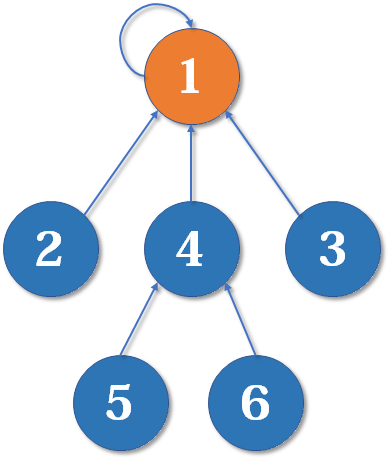
A disjoint-set union is a that dynamically maintains several disjoint sets data structure, and supports two main operations:

Operation	Description
find(x)	Find elementsxthe representative (root node) of the set it belongs to
union(x, y)/join(x, y)	merge the sets to which two elements belong
(optional)connected(x, y)	determine whether two elements belong to the same set (i.e.find(x) == find(y)）

Data structure definition

#include <vector>
#include <algorithm>

using std::vector;

class DSU {
    public:
	vector<int> parent; // the parent node of each node
	vector<int> rank; // (optional) used for union by rank or to record set size

	DSU(int n)
	{
		parent.resize(n);
		rank.resize(n, 0);
		for (int i = 0; i < n; i++) {
			parent[i] = i;
		}
	}

	int find(int x)
	{
		// Path compression, making the find complexity close to O(1)
		if (parent[x] != x) {
			parent[x] = find(parent[x]);
		}
		return parent[x];
	}

	void join(int x, int y)
	{
		// Union by rank
		int rootX = find(x);
		int rootY = find(y);
		if (rootX == rootY) {
			return;
		}

		if (rank[rootX] < rank[rootY]) { //the one with the larger rank among the two sets is rootX
			std::swap(rootX, rootY);
		}

		parent[rootY] = rootX;//the one with smaller rank is attached under the one with larger rank

		if (rank[rootX] == rank[rootY]) { //if the two sets have equal rank, the rank of the merged set is increased by 1
			rank[rootX]++;
		}
	}

	bool connected(int x, int y)
	{
		return find(x) == find(y);
	}
};

Techniques:

technology	Description	Effect
Path Compression	Beforefind()when finding, point the parent of all nodes on the search path to the root node	significantly reduces tree height, almost amortized O(1)
Union by Rank/Size	Beforeunion()when [unioning], attach the ‘short tree’ under the ‘tall tree’	keeps the tree balanced, further optimizing search efficiency

Time complexity

Operation	amortized time complexity
find()	approximately O(1)
union()	approximately O(1)
connected()	approximately O(1)

Strictly speaking, it is O(α(n)), but α(n) ≤ 5 for any practically sized n.

string

string pattern matching

The positioning operation of a substring is usually called the string’spattern matching, which finds the position of the substring (usually called the pattern string) in the main string.

naive pattern matching algorithm

pattern stringpand the main strings

S: a b a b c a b c a c b a b
P: a b c a c
   ↑ 从这里开始和主串对齐

步骤1：
S: a b a b c a b c a c b a b
P: a b c a c
   a = a ✅
     b ≠ a ❌ 失配 → 模式右移一位

步骤2：
S: a b a b c a b c a c b a b
  P: a b c a c
     a ≠ b ❌ → 继续右移一位

步骤3：
S: a b a b c a b c a c b a b
    P: a b c a c
       a = a ✅
         b = b ✅
           c = a ❌ → 右移一位

步骤4：
S: a b a b c a b c a c b a b
      P: a b c a c
         b ≠ a ❌ → 右移一位

步骤5：
S: a b a b c a b c a c b a b
        P: a b c a c
           c = a ❌ → 右移一位

步骤6：
S: a b a b c a b c a c b a b
          P: a b c a c
             a = a ✅
               b = b ✅
                 c = c ✅
                   a = a ✅
                     c = c ✅ ✅ 匹配成功！

Code:

#include <stdio.h>
#include <string.h>

int naive_match(const char *s, const char *p) {
    int i=0,j=0;
    int s_len = strlen(s);
    int p_len = strlen(p);

	while(i<s_len && j<p_len){
        if(s[i]==p[j]){
            i++;
            j++;
        }else{
            i = i - j + 1;//backtrack and re-match
            j = 0;
        }
    }
    if(j == p_len){
        return i - j;
    }
    return -1; 
}

worst case：$O(n \cdot m)$, where $n$ is the length of the main string,$m$ is the length of the pattern string.

• for example, the main string"aaaaaaab"and the pattern string"aaaab", each time a match fails, it needs to backtrack multiple characters.

average case: usually less than the worst case, but may still approach $O(n \cdot m)$。

KMP algorithm

Recommended article with a very good explanation:

Thoroughly understand from beginning to endKMP

https://www.cnblogs.com/JoBlg/p/4087230.html?tdsourcetag=s_pctim_aiomsg

In the naive pattern matching algorithm, each time a match fails, the pattern string (the substring to be matched) is shifted one position and comparison starts from the beginning.

Several concepts:

• Prefix: all substrings that include the first character but exclude the last character
• Suffix: all substrings that include the last character but exclude the first character
• PM(Partial Match) Partial match value, i.e., the table below

Below, take “ABCDABD” as the substring to be matched as an example:

Substring	Prefix set (excluding the full string)	Suffix set (excluding the full string)	Length of the longest equal prefix and suffix
A	(Empty)	(Empty)	0
AB	A	B	0
ABC	A, AB	C, BC	0
ABCD	A, AB, ABC	D, CD, BCD	0
ABCDA	A, AB, ABC, ABCD	A, DA, CDA, BCDA	1（A）
ABCDAB	A, AB, ABC, ABCD, ABCDA	B, AB, DAB, CDAB, BCDAB	2 (AB)
ABCDABD	A, AB, ABC, ABCD, ABCDA, ABCDAB	D, BD, ABD, DABD, CDABD, BCDABD	0

Then the PM table is

Number	0	1	2	3	4	5	6
String[i]	A	B	C	D	A	B	D
PM	0	0	0	0	1	2	0

• If the text string “BBC ABCDAB ABCDABCDABDE” and the pattern string “ABCDABD” are given, and now we want to match the pattern string against the text string, as shown in the figure below:

img

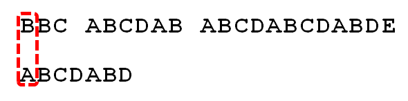
• 1. Because the character A in the pattern string does not match the characters B, B, C, and space in the text string at the beginning, there is no need to apply the conclusion; just keep shifting the pattern string right by one position until the character A in the pattern string successfully matches the 5th character A in the text string:

img

• 2. Continue matching forward. When the last character D of the pattern string mismatches while matching against the text string, it is obvious that the pattern string needs to move to the right. But how many positions to the right? Because the number of matched characters at this point is 6 (ABCDAB), and then according toPMFrom the table, the length value corresponding to the character B before the mismatched character D is 2, so according to the previous conclusion, it needs to move right by 6 - 2 = 4 positions, fromPM[i] = 2 i.e., restart matching at the position with index 2

img

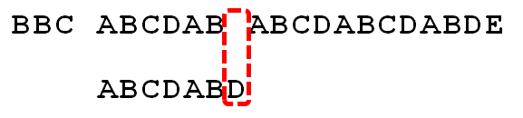
We can define anextarray: when the j-th character (0-based) of the pattern string fails to match, continue matching from the next[j]-th character of the pattern string.

The next array in KMPThere are two ways of writing it:

PM table = prefix function π(i)(also calledlps array，Longest Prefix Suffix）。

• In some textbooks, next is equal to PM (lps)

• In some textbooks, next is a variant of PM

  • next[0] = -1 (meaning to restart matching from the very beginning)

  • next[i] = PM[i-1]

#include <string.h>

void GetNext(char *p, int next[])
{
	int pLen = strlen(p);
	next[0] = -1;
	int k = -1;
	int j = 0;
	while (j < pLen - 1) {
		//p[k] represents the prefix, p[j] represents the suffix
		if (k == -1 || p[j] == p[k]) {
			++k;
			++j;
			next[j] = k;
		} else {
			k = next[k];
		}
	}
}

int KmpSearch(char *s, char *p, int next[])
{
	int i = 0;
	int j = 0;
	int sLen = strlen(s);
	int pLen = strlen(p);
	while (i < sLen && j < pLen) {
		//If j = -1, or the current character matches successfully (i.e., S[i] == P[j]), then increment i and j
		if (j == -1 || s[i] == p[j]) {
			i++;
			j++;
		} else {
			//If j != -1 and the current character match fails (i.e., S[i] != P[j]), then keep i unchanged and set j = next[j]
			//next[j] is the next value corresponding to j
			j = next[j];
		}
	}
	if (j == pLen)
		return i - j;
	else
		return -1;
}

Trees and Binary Trees

Terminology

graph TD A[A] --> B[B] A --> C[C] B --> D[D] B --> E[E] C --> F[F] C --> G[G] E --> H[H] E --> I[I] style A fill:#f9f,stroke:#333,stroke-width:2px style D fill:#9f9,stroke:#333 style F fill:#9f9,stroke:#333 style G fill:#9f9,stroke:#333 style H fill:#9f9,stroke:#333 style I fill:#9f9,stroke:#333

• Node Classification

  • Root node

    • The topmost node of the tree.

    • Example:Ais the root node.

  • Parent

    • The node directly above a node.

    • Example:Bis the parent node ofA。

  • Sibling

    • Nodes that have the same parent are siblings.

    • Example:DandEare siblings,FandGare siblings.

  • Child node

    • Child node: a node directly connected to the parent node.
    • Example:D、EYesBthe child node of.

  • Descendants

    • All descendants of a node, including child nodes.
    • Example:H、IYesBthe descendants of.

  • Branch node (Internal Node)

    • A node that has child nodes.
    • Example:A、B、C、Eare all branch nodes.

  • Leaf node

    • A node without child nodes.
    • Example:D、F、G、H、IIt is a leaf node.

• Node Attributes

  • Depth of a Node

    • The path length (number of edges) from the root node to this node. (Top-down)

    • Example:ADepth 0,BDepth 1,DDepth 2.

  • Height of a Node

    • The length of the longest path from this node to the deepest leaf node. (Bottom-up)

    • Example:BHeight 2 (longest path B→E→H or B→E→I).

    • Level of a Node

      • Level = Depth + 1

      • Example: Root node A is level 1, B is level 2.

    • Degree

      • The number of child nodes a node has.
      • Example:Bhas degree 2 (D、E）。

• Tree Classification

  • Tree of degree m

    • The degree of any node is not greater than m.
    • At least one node has degree m.
    • It must be a non-empty tree, so it has at least m+1 nodes.

  • m-ary tree

    • The degree of any node is not greater than m.
    • It can be an empty tree.

  • Ordered Tree / Unordered Tree

    • Ordered Tree: The subtrees of each node in the tree are ordered from left to right and cannot be interchanged; that is, the child nodes have a fixed order.

    • Unordered Tree: The order of child nodes is not important.

  • Forest

    • A collection of multiple trees that are not connected to each other.

    • If the root node A is removed, two trees, B and C, are formed, making a forest.

• Other Concepts

  • Path
    • The sequence of nodes traversed from one node to another.
    • Example: A→B→E→H is a path.
  • Path Length
    • The number of edges on the path.
    • Example: A→B→E→H, path length = 3.

Properties of Trees

1. The number of nodes in a tree equals the sum of the degrees of all nodes plus 1.

   • The proof is simple: except for the root node, every other node has one edge above it.

2. A tree of degree $m$ the tree’s $i$ level has at most $m^{i-1}$ nodes ($i \ge 1$)

3. A tree of height $h$ of $m$ ary tree has at most $\frac{m^h-1}{m-1}$ nodes

4. Having $n$ nodes $m$ The minimum height of an m-ary tree is $\lceil \log_m(n(m-1)+1) \rceil$

   • Proof: In the case of minimum height, try to make every node have $m$ children, then:
   • $\frac{m^{h-1}-1}{m-1} < n \le \frac{m^h-1}{m-1}$

Binary Tree

A binary tree is an ordered tree.

Terminology

• Full binary tree

  graph TD style A fill:#f9f,stroke:#333,stroke-width:2px style B fill:#9cf,stroke:#333,stroke-width:1px style C fill:#9cf,stroke:#333,stroke-width:1px style D fill:#9cf,stroke:#333,stroke-width:1px style E fill:#9cf,stroke:#333,stroke-width:1px style F fill:#9cf,stroke:#333,stroke-width:1px style G fill:#9cf,stroke:#333,stroke-width:1px style H fill:#9f9,stroke:#333,stroke-width:1px style I fill:#9f9,stroke:#333,stroke-width:1px style J fill:#9f9,stroke:#333,stroke-width:1px style K fill:#9f9,stroke:#333,stroke-width:1px style L fill:#9f9,stroke:#333,stroke-width:1px style M fill:#9f9,stroke:#333,stroke-width:1px style N fill:#9f9,stroke:#333,stroke-width:1px style O fill:#9f9,stroke:#333,stroke-width:1px A((1)) --> B((2)) A --> C((3)) B --> D((4)) B --> E((5)) C --> F((6)) C --> G((7)) D --> H((8)) D --> I((9)) E --> J((10)) E --> K((11)) F --> L((12)) F --> M((13)) G --> N((14)) G --> O((15))

  • with height $h$ , and a binary tree containing $2^h-1$ nodes is called a full binary tree.

  • In a full binary tree, every node except leaf nodes has degree 2.

  • A full binary tree can be numbered in level order., for the node numbered $i$ :

    • Left child number:$2i$

    • Right child number:$2i+1$

    • Parent node number:$\lfloor i/2 \rfloor$

• Complete binary tree

  graph TD style A fill:#f9f,stroke:#333,stroke-width:2px style B fill:#9cf,stroke:#333,stroke-width:1px style C fill:#9cf,stroke:#333,stroke-width:1px style D fill:#9cf,stroke:#333,stroke-width:1px style E fill:#9cf,stroke:#333,stroke-width:1px style F fill:#9cf,stroke:#333,stroke-width:1px style G fill:#9cf,stroke:#333,stroke-width:1px style H fill:#9f9,stroke:#333,stroke-width:1px style I fill:#9f9,stroke:#333,stroke-width:1px style J fill:#9f9,stroke:#333,stroke-width:1px style K fill:#9f9,stroke:#333,stroke-width:1px style L fill:#9f9,stroke:#333,stroke-width:1px A((1)) --> B((2)) A --> C((3)) B --> D((4)) B --> E((5)) C --> F((6)) C --> G((7)) D --> H((8)) D --> I((9)) E --> J((10)) E --> K((11)) F --> L((12))
  • with height$h$, with$n$nodes, if and only if each of its nodes corresponds one-to-one with the nodes in a full binary tree of height$h$full binary tree, when they correspond one-to-one with the nodes numbered 1 to n, it is called a complete binary tree.
  • If $i \le \lfloor \frac{n}{2} \rfloor$, then node $i$ is a branch node.
  • Leaf nodes can only appear in the largest two levels. For leaf nodes at the largest level, they are all arranged in order at the leftmost positions of that level.
  • If there is a node with degree 1, there can be only one, and that node has only a left child but no right child.
  • After level-order numbering, once a node (numbered $i$ ) is a leaf node or has only a left child, then nodes numbered greater than $i$ are all leaf nodes.
  • If $n$ if it is odd, then every branch node has both a left child and a right child; if $n$ if it is even, then the branch node with the largest number (numbered $\frac{n}{2}$ ) has only a left child and no right child, while the remaining nodes have both left and right children
  • Of the two subtrees of a complete binary tree (the left and right subtrees of the root), at least one is a full binary tree

• Binary Search Tree

  • The keys of all nodes in the left subtree are smaller than the key of the root node, and the keys of all nodes in the right subtree are greater than the key of the root node; both the left and right subtrees are also binary search trees.

• Balanced Binary Tree

  • on the treethe difference between the depths of the left subtree and the right subtree of any node does not exceed 1

English Definition

Properties

1. The number of leaf nodes in a non-empty binary tree equals the number of nodes with degree 2 plus 1, i.e., $n_0 = n_2+1$

2. On the $k$-th level of a non-empty binary tree, there are at most $2^{(k-1)}$ nodes ($k \ge 1$)

3. with height $h$ has at most $2^h-1$ nodes ($h\ge1$）

4. with $n$ nodesComplete binary treehas height $\lceil \log_2(n+1) \rceil$ or $\lfloor \log_2 n \rfloor + 1$

5. forComplete binary treeNumber the nodes, and the following relationships hold

Item	1-based numbering(root=1)	0-based numbering(root=0)
Left child	$\text{left}(i)=2i$	$\text{left}(i)=2i+1$
Right child	$\text{right}(i)=2i+1$	$\text{right}(i)=2i+2$
Parent node	$\text{parent}(i)=\lfloor i/2 \rfloor（i>1）$	$\text{parent}(i)=\lfloor (i-1)/2 \rfloor（i>0）$
Condition for having at least a left child	$2i \le n$	$2i+1 < n$
Condition for right child existence	$2i+1 \le n$	$2i+2 < n$
Leaf node condition	$i > \lfloor n/2 \rfloor$	$i > \lfloor (n-2)/2 \rfloor$ or $2i+1 \ge n$
Condition for having only a left child	$2i = n$	$2i+1 < n$ and $2i+2 \ge n$
Depth (root level=1)	$\lfloor \log_2 i \rfloor +1$	$\lfloor \log_2 (i+1) \rfloor +1$
Depth (root level=0)	$\lfloor \log_2 i \rfloor$	$\lfloor \log_2 (i+1) \rfloor$

Storage structure

• Sequential Storage Structure

Array storage: store according to the complete binary tree method, using 0 or -1 to represent empty nodes.

• Linked Storage

It is easy to verify that in a binary linked list containing$n$nodes, there are $n+1$null pointer fields

With n nodes, there are 2n pointer fields; n-1 nodes have a pointer pointing to them, so there are n+1 null pointer fields

Binary tree traversal

Preorder traversal

Visit the root node first, then traverse the left subtree, then traverse the right subtree

Recursive implementation

void PreOrder(BiTree T){
    if(T!=NULL){
        visit(T);
        PreOrder(T->lchild);
        PreOrder(T->rchild);
    }
}

Non-recursive implementation

void PreOrder(BiTree T){
	Stack *S;
    InitStack(S);
    BiTree p = T;
    while(p || !isEmpty(S)){//Loop while the stack is not empty or p is not null
        if(p){
            visit(p);
            Push(S, p);
            p = p->lchild;
        }else{
            Pop(S, p);
            p = p->rchild;
        }
        
    }
    DestroyStack(S);
}

Rust language description

// Definition for a binary tree node.
#[derive(Debug, PartialEq, Eq)]
pub struct TreeNode {
    pub val: i32,
    pub left: Option<Rc<RefCell<TreeNode>>>,
    pub right: Option<Rc<RefCell<TreeNode>>>,
}

impl TreeNode {
    #[inline]
    pub fn new(val: i32) -> Self {
        TreeNode {
            val,
            left: None,
            right: None,
        }
    }
}


use std::cell::RefCell;
use std::rc::Rc;

pub fn preorder(root: &mut Option<Rc<RefCell<TreeNode>>>, visit:  &impl Fn(&mut Rc<RefCell<TreeNode>>)) {
    // Preorder traversal
    let mut stack = Vec::new();
    let mut p = root.clone();

    // Preorder traversal
    while let Some(node) = p {
        visit(node);
        // Push the right child onto the stack
        if let Some(right) = node.borrow().right.clone() {
            stack.push(right);
        }
        // Push the left child onto the stack; if the left child is empty, pop the stack, otherwise p = Some(left)
        if let Some(left) = node.borrow().left.clone() {
            p = Some(left);
        } else {
            p = stack.pop();
        }
    }
}

Inorder traversal

Traverse the left subtree first, then visit the root node, then traverse the right subtree

Recursive implementation

void InOrder(BiTree T){
    if(T!=NULL){
        InOrder(T->lchild);
        visit(T);
        InOrder(T->rchild);
    }
}

Non-recursive implementation

1. Starting from the left child of the root, push nodes onto the stack one by one until the left child is null, indicating that a node that can be output has been found
2. Pop the top element from the stack and visit it; if it has a right child, continue with step 1; otherwise continue with step 2

void InOrder(BiTree T){
	Stack *S;
    InitStack(S);
    BiTree p = T;
    while(p || !isEmpty(S)){//Loop while the stack is not empty or p is not null
        if(p){
            Push(S, p);
            p = p->lchild;
        }else{
            Pop(S, p);
            visit(p);
            p = p->rchild;
        }
        
    }
    DestroyStack(S);
}

Postorder traversal

Traverse the left subtree first, then the right subtree, then visit the root node

Recursive implementation

void PostOrder(BiTree T){
    if(T!=NULL){
        PostOrder(T->lchild);
        PostOrder(T->rchild);
        visit(T);
    }
}

Non-recursive implementation

1. Starting from the left child of the root, push nodes onto the stack one by one until the left child is null;
2. Read the top element of the stack: if its right child is not null and has not been visited, perform step 1 on the right subtree; otherwise, pop the top element and visit it

If the top element of the stack is to be popped and visited, either its right subtree is empty, or its right subtree has already been fully visited (at this time the left subtree has long been visited). Therefore we need an auxiliary pointer to indicate the most recently visited node:

void PostOrder(BiTree T){
	Stack *S;
    InitStack(S);
    BiTNode *p = T;
    BiTNode *r= NULL;
    while(p || !isEmpty(S)){//Loop while the stack is not empty or p is not null
        if(p){
            Push(S, p);
            p = p->lchild;
        }else{
            GetTop(S,p);
            if(p->rchild && p->rchild != r){
                p = p->rchild;
            }else{
                Pop(S, p);
            	visit(p);
                r = p;
            	p = NULL;
            }
        }
        
    }
    DestroyStack(S);
}

In postorder traversal, when about to visit a node, the nodes in the stack at that time are all the nodes on the path from root to the current node.

Non-recursive implementations of the three traversals

#include <vector>
#include <stack>
using std::vector;
using std::stack;

struct TreeNode {
        int val;
        TreeNode *left;
        TreeNode *right;
        TreeNode()
                : val(0)
                , left(nullptr)
                , right(nullptr)
        {
        }
        TreeNode(int x)
                : val(x)
                , left(nullptr)
                , right(nullptr)
        {
        }
        TreeNode(int x, TreeNode *left, TreeNode *right)
                : val(x)
                , left(left)
                , right(right)
        {
        }
};

vector<struct TreeNode *> preorder_traverse(struct TreeNode *root)
{
        stack<struct TreeNode *> stk;
        TreeNode *p = root;
        vector<struct TreeNode *> ret;

        while (p || !stk.empty()) {
                if (p) {
                        ret.push_back(p); // visit p
                        stk.push(p);
                        p = p->left;
                } else {
                        p = stk.top();
                        stk.pop();
                        p = p->right;
                }
        }
        return ret;
}

vector<struct TreeNode *> inorder_traverse(struct TreeNode *root)
{
        stack<struct TreeNode *> stk;
        TreeNode *p = root;
        vector<struct TreeNode *> ret;

        while (p || !stk.empty()) {
                if (p) {
                        stk.push(p);
                        p = p->left;
                } else {
                        p = stk.top();
                        stk.pop();
                        ret.push_back(p); // visit p
                        p = p->right;
                }
        }
        return ret;
}

vector<struct TreeNode *> postorder_traverse(struct TreeNode *root)
{
        stack<struct TreeNode *> stk;

        TreeNode *p = root, *last = nullptr;
        vector<struct TreeNode *> ret;

        while (p || !stk.empty()) {
                if (p) {
                        stk.push(p);
                        p = p->left;
                } else {
                        p = stk.top();
                        if (p->right != nullptr && p->right != last) {
                                p = p->right;
                        } else {
                                stk.pop();
                                ret.push_back(p); // visit p
                                last = p;
                                p = nullptr;
                        }
                }
        }

        return ret;
}

Level-order traversal

Traverse in order from the first level to the last level, from left to right

void LevelOrder(BiTree T){
    Queue *Q;
    InitQueue(Q);
    EnQueue(Q, T);
    while(!isEmpty(Q)){
        DeQueue(Q,p);
        visit(p);
        if(p->lchild!=NULL){
            EnQueue(Q, p->lchild);
        }
        if(p->rchild!=NULL){
            EnQueue(Q, p->rchild);
        }
    }
    DestroyQueue(Q);
}

If you need to record or perform some operations when each level has been visited:

/**
 * Definition for a binary tree node.
 **/
struct TreeNode {
	int val;
	TreeNode *left;
	TreeNode *right;
	TreeNode()
		: val(0)
		, left(nullptr)
		, right(nullptr)
	{
	}
	TreeNode(int x)
		: val(x)
		, left(nullptr)
		, right(nullptr)
	{
	}
	TreeNode(int x, TreeNode *left, TreeNode *right)
		: val(x)
		, left(left)
		, right(right)
	{
	}
};
#include <vector>
#include <queue>
using std::vector;
using std::queue;

class Solution {
    public:
	vector<int> rightSideView(TreeNode *root)
	{
		int i, n;
		vector<int> res;
		queue<TreeNode *> que;
		TreeNode *p;
		if (root == nullptr) {
			return res;
		}
		que.push(root);

		while (!que.empty()) {
			n = que.size();
			res.push_back(que.back()->val);
			for (i = 0; i < n; i++) {
				p = que.front();
				if (p->left) {
					que.push(p->left);
				}
				if (p->right){
				que.push(p->right);
				}
				que.pop();
			}
		}
		return res;
	}
};

Morris Traversal

Morris traversal uses the idea of threaded binary trees. In the Morris method, there is no need to allocate additional pointers for each node to point to its predecessor or successor; it only needs to use the left and right null pointers in leaf nodes to point to the predecessor or successor node under a certain traversal order.

graph TD subgraph 图2 B1[1] B2[2] B3[3] B4[4] B5[5] B6[6] B7[7] B1 --> B2 B1 --> B3 B2 --> B4 B2 --> B5 B3 --> B6 B3 --> B7 B4 -.-> B2:::cur2 B5 -.-> B1:::cur1 B6 -.-> B3:::curn end subgraph 图1 A1[1] --> A2[2] A1 --> A3[3] A2 --> A4[4] A2 --> A5[5] A3 --> A6[6] A3 --> A7[7] end

The overall idea of Morris is to start with a certain root node,find the rightmost node of its left subtree and connect it to this root node.

We can see from Figure 2 that after connecting in this way, the cur pointer can completely traverse from one node to the next, traversing the entire tree until node 7 has no right pointer. Code example:

/**
 * Definition for a binary tree node.
 **/
struct TreeNode {
        int val;
        TreeNode *left;
        TreeNode *right;
        TreeNode()
                : val(0)
                , left(nullptr)
                , right(nullptr)
        {
        }
        TreeNode(int x)
                : val(x)
                , left(nullptr)
                , right(nullptr)
        {
        }
        TreeNode(int x, TreeNode *left, TreeNode *right)
                : val(x)
                , left(left)
                , right(right)
        {
        }
};

extern void visit(TreeNode *root);

class Solution {
    private:
    public:
        void preOrderMorris(TreeNode *root)
        {
                if (root == nullptr)
                        return;

                TreeNode *curr = root; // current node
                TreeNode *curr_left = nullptr; // the root node of the current node's left subtree

                while (curr != nullptr) {
                        curr_left = curr->left;

                        if (curr_left == nullptr) {
                                visit(curr);
                                curr = curr->right; // In the phase of returning to the upper level, keep moving right.
                        } else {
                                // Find the rightmost node of the current left subtree, and do not return to the upper level along the connection.
                                while (curr_left->right != nullptr && curr_left->right != curr)
                                        curr_left = curr_left->right;
                                // If the right pointer of the rightmost node does not point to the root node, create a connection and proceed to connect to the root node of the next left subtree.
                                if (curr_left->right == nullptr) {
                                        visit(curr);
                                        curr_left->right = curr;
                                        curr = curr->left;
                                } else {
                                        // When the rightmost node of the left subtree points to the root node, it indicates that we have entered the phase of returning to the upper level,
                                        // It is no longer the initial connection-building phase. At the same time, when returning to the root node, we should have already processed the lower-level nodes, so we can simply disconnect the connection.
                                        curr_left->right = nullptr;
                                        curr = curr->right; // In the phase of returning to the upper level, keep moving right.
                                }
                        }
                }
        }
};

#include <iostream>
using std::cout;
void visit(TreeNode *root)
{
        cout << root->val << " ";
}

int main()
{
        /*
            4
           / \
          2   6
         / \ / \
        1  3 5  7
       */

        TreeNode *n1 = new TreeNode(1);
        TreeNode *n3 = new TreeNode(3);
        TreeNode *n5 = new TreeNode(5);
        TreeNode *n7 = new TreeNode(7);

        TreeNode *n2 = new TreeNode(2, n1, n3);
        TreeNode *n6 = new TreeNode(6, n5, n7);

        TreeNode *root = new TreeNode(4, n2, n6);

        Solution sol;

        cout << "Morris Preorder Traversal: ";
        sol.preOrderMorris(root);
        cout << '\n';

        return 0;
}

Graph

Terminology

Basic Concepts

Terminology	Explanation
Directed Graph	The edges in the graph have directions, such as $A \rightarrow B$
Undirected Graph	Edges have no direction, such as $A - B$, indicating a bidirectional relationship

Classification by Edge Structure

Terminology	Explanation
Simple Graph	Not allowed self-loop(connecting to itself) and multiple edges(multiple edges between two vertices)
Multigraph	Allows self-loops and multiple edges

---

Special Graphs

Terminology	Explanation
Complete Graph	There is an edge between any two vertices. An undirected complete graph is denoted as $K_n$, with $\frac{n(n-1)}{2}$ edges
Subgraph	A graph formed by taking some vertices and edges from the original graph

Graph Connectivity

Terminology	Explanation
Connected	In an undirected graph, any two vertices are connected by a path
Connected graph	The graph is connected as a whole
Connected component	A maximal connected subgraph in an undirected graph (a connected piece that cannot be enlarged)
Strongly connected graph	In a directed graph, any two vertices $u$ and $v$ there exist mutually reachable paths
Strongly connected component	The largest strongly connected subgraph in a directed graph

Tree-related

Terminology	Explanation
Spanning Tree	In a connected undirected graph, contains all vertices and has the minimum number of edges ($n-1$) tree
Spanning Forest	For a disconnected graph, a set of spanning trees generated from each connected component.

Vertex and edge properties

Terminology	Explanation
Degree of a vertex	Number of edges connected to a vertex (in an undirected graph)
In-degree	Number of edges pointing to the vertex in a directed graph
Out-degree	Number of edges pointing out from the vertex in a directed graph
Edge weight	A value attached to an edge (such as distance, time, cost, etc.)
Network	A weighted graph (a graph with edge weights) is also called a network.
Dense Graph	A graph with many edges; a vague concept.
Sparse Graph	A graph with few edges; a vague concept.

Paths and distances

Terminology	Explanation
path	A sequence of vertices in which any two adjacent vertices are connected by an edge.
Path length	The number of edges on the path (or the sum of weights).
Cycle	A path with the same start and end
Simple path	Vertices in the path are not repeated
Simple cycle	In a cycle, no vertices are repeated except the start and end
Distance	The length of the shortest path between two vertices

Store

Adjacency matrix method

Undirected graph：

• ifiandjIf there is an edge:Edge[i][j] = Edge[j][i] = 1
• If there is no edge:Edge[i][j] = Edge[j][i] = 0

Directed graph：

• If there isi → jan edge:Edge[i][j] = 1
• If there is no edge:Edge[i][j] = 0

Network (weighted graph)：

• ifi → jthe weight of … isw, thenEdge[i][j] = w

• When there is no edge, it is generally set to∞(or a very large number)

• C language description

#define MaxVertexNum 100
typedef char VertexType;
typedef int EdgeType;
typedef struct{
    VertexType Vex[MaxVertexNum];              // Vertex table
    EdgeType Edge[MaxVertexNum][MaxVertexNum]; //Adjacency matrix
}MGraph;

• C++ description

#include <unordered_map>
#include <vector>
using std::unordered_map;
using std::vector;

// The range of node indices is not fixed
unordered_map<int, vector<int>> graph;
// Determining the range of node indices
vector<vector<int>> graph;

Adjacency list method

• C language description

#define MaxVertexNum 100
typedef struct ArcNode{//Edge table node
    int adjvex; //The vertex pointed to by the arc
    struct ArcNode *next;
    // InfoType info // edge weight
}ArchNode;

typedef struct VNode{//Vertex table node
    VertexType data; // vertex information
    ArchNode *first; //Pointer to the first arc incident to the vertex
}VNode,AdjList[MaxVertexNum];

typedef struct{
    AdjList vertices;/// adjacency list
    int vexnum, arcnum;
}ALGraph;

• C++ description

Orthogonal linked list method

#define MaxVertexNum 100

typedef struct ArcNode {
    int tailvex;             // Arc tail (starting point)
    int headvex;             // Arc head (end point)
    struct ArcNode *hlink;   // Pointer to the next arc with the same head
    struct ArcNode *tlink;   // Pointer to the next arc with the same tail
    int info;                // Weight (optional)
} ArcNode;

typedef struct VexNode {
    char data;               // vertex information
    ArcNode *firstin;        // Pointer to the first incoming arc
    ArcNode *firstout;       // Pointer to the first outgoing arc
} VexNode;

typedef struct {
    VexNode xlist[MaxVertexNum]; // Vertex table
    int vexnum, arcnum;          // Number of vertices, number of arcs
} OLGraph; // Orthogonal List Graph

Adjacency multilist

Adjacency multilist is another linked storage structure for undirected graphs

typedef struct ENode {
    int ivex, jvex;                 // The indices of the two vertices of the edge
    struct ENode *ilink, *jlink;   // point to the next edges incident to ivex and jvex respectively
} ENode;

typedef struct VNode {
    char data;                     // vertex information
    ENode *firstedge;             // the first edge incident to this vertex
} VNode;

typedef struct {
    VNode adjList[MaxVertexNum];
    int vexnum, edgenum;
} AMLGraph;  // Adjacency Multilist: Adjacency Multilist Graph

Graph traversal

Breadth-First Search

bool visited[MAX_VERTEX_NUM];

void BFSTraverse(Graph G) {
    Queue *Q;
    for(i = 0;i < G.vexnum;i++){
        visited[i] = false;
    }
    InitQueue(Q);
	for(i = 0;i < G.vexnum;i++){//Call BFS for each connected component
        if(!visited[i]){
            BFS(G,i);
        }
    }   
    DestroyQueue(Q);
}

void BFS(Graph G, int v){//Starting from vertex v, perform breadth-first traversal of G
    visit(v);
    visited[v] = TRUE;
    Enqueue(Q, v);
    while(!isEmpty(Q)){
        DeQueue(Q,v);
        for(w = FirstNeighbor(G,v);w>=0;w=NextNeighbor(G,v,w)){ //Enqueue all unvisited neighbors of v
            if(!visited[w]){
                visit(w);
                visited[w] = true;
                EnQueue(Q,w);
            }
        }
    }
}

If the graph is unweighted, BFS can be used to solve the single-source shortest path problem, mainly by exploiting the property that breadth-first traversal visits vertices in order of increasing distance from the source.

Depth-First Search

Recursive form

bool visited[MAX_VERTEX_NUM];
void DFSTraverse(Graph G){
    for(v = 0;v<G.vexnum;v++)
        visited[v]=false;
        
    for(v = 0;v<G.vexnum;v++){
        if(!visited[v])
            DFS(G,v);
    }
}
void DFS(Graph G, int v){
    visit(v);
    visited[v] = true;
  	for(w = FirstNeighbor(G,v); w>=0 ; w = NextNeighbor(G,v,w)){
        if(!visited[w]){
            DFS(G,w);
        }
    }
}

Non-recursive form

void DFS_Non_RC(AGraph &G, int v){
    int w;
    Stack *S;
    InitStack(S);
    for(i = 0;i<G.num;i++)
        visited[i] = false;

    Push(S,v);
    visited[v] = true;//Indicates already pushed onto the stack.
    while(!isEmpty(S)){
        k = Pop(S);
        visit(k);
        for(w = FirstNeighbor(G,k);w>=0;w=NextNeighbor(G,k,w)){
           if(!visited[w]){
               Push(S,w);
               visited[w] = true;
           } 
        }
        
    }
    DestroyStack(S);
}

Minimum Spanning Tree

Prim’s algorithm

Idea: Starting from one vertex, each time selectthe edge with the minimum costAdd the new vertex to the spanning tree

More suitable for：dense graphs(adjacency matrix)

Kruskal’s algorithm

Idea: Sort all edges of the graph by weight, select edges from smallest to largest, as long asno cycle is formedthen choose

Suitable for：sparse graph

uses union-findavoid forming cycles

shortest path

Dijkstra’s algorithm

single-source shortest path problem

Floyd’s algorithm

shortest paths between all pairs of vertices

Topological Sort

Take the following problem as an example:

P207 Course Schedule

https://even629.com/posts/207

#include <vector>
#include <queue>

using std::vector;
using std::queue;

class Solution {
    public:
        bool canFinish(int numCourses, vector<vector<int> > &prerequisites)
        {
                // Build the graph
                int i;
                vector<vector<int> > graph(numCourses);
                vector<int> indegree(numCourses, 0); // Store the in-degree of each node
                vector<bool> pushed(numCourses, false);
                queue<int> que;

                for (vector<int> &vec : prerequisites) {
                        graph[vec[1]].push_back(vec[0]);
                        indegree[vec[0]]++;
                }

                // Topological Sort
                // During initialization, first add the vertices with in-degree 0.
                for (i = 0; i < numCourses; i++) {
                        if (indegree[i] == 0) {
                                que.push(i);
                                pushed[i] = true;
                        }
                }

                while (!que.empty()) {
                        i = que.front();
                        que.pop();

                        // Each time, find a vertex with in-degree 0.
                        for (int course : graph[i]) {
                                indegree[course]--;

                                if (!pushed[course] && indegree[course] == 0) {
                                        que.push(course);
                                        pushed[course] = true;
                                }
                        }
                }

                for (i = 0; i < numCourses; i++) {
                        if (!pushed[i])
                                return false;
                }

                return true;
        }
};

critical path

Hash

Reference article:

Thoroughly Understanding Hash Tables(HashTable)Structure

https://blog.csdn.net/qq_45730399/article/details/143592213

Hash table (Hash Table) also known as a hash table is a data structure that uses key-value pairs (Key-Value Pair) to store data, andBy mapping keys to specific positions in an array via a hash function, it enables efficient lookup, insertion, and deletion operations.

Concept

• Storage structure: A hash table usually consists of an array and a hash function. Each element of the array is called a bucket, which can store one or more key-value pairs.

• Hash function : The hash function converts a key into an array index (i.e., an integer).

• Hashing: It is the process of converting input data (usually of arbitrary length) into a fixed-length output (an index within the array range) using a hash function.

• Hash Collision : When different keys are mapped to the same index by a hash function, a hash collision occurs. Common methods to resolve hash collisions include chaining and open addressing.

• Load Factor：The ratio of the number of elements stored in the hash table to the array size (total number of slots).

  • The size of the hash table (number of slots) is fixed, but the number of stored elements can exceed the number of slots.
  • The load factor represents the utilization efficiency of hash table space.A higher load factor means more elements are stored in the table, and space utilization is high.
  • whenWhen the load factor increases (close to 1 or higher), the lookup efficiency of the hash table may decrease., especially when using open addressing, collision resolution requires more probing attempts.
  • When using chaining, an increase in the load factor leads to longer linked lists, thereby increasing the average lookup time.
  • In a dynamic hash table, when the load factor exceeds a certain threshold (e.g., 0.75), the hash table is usually resized (expanded) to reduce collisions and improve performance.
  • If the load factor is too low, it may lead to shrinking (capacity reduction) to save space.
  • Ideal load factor:
    • Open addressing: The ideal load factor is usually below 1, recommended between 0.5 and 0.75, to balance space utilization and lookup efficiency.
    • Chaining: The load factor can exceed 1 because multiple elements can be stored in the same slot. Usually a load factor between 0.7 and 1.0 is a good choice, but it can be higher, depending on the impact of linked list length on performance.

• Rehashing: When the load factor of the hash table exceeds a set value, expansion may be necessary. Expansion usually involves creating a larger array and recalculating the hash values of all keys to map them into the new array.

• Shrinkage: Shrinking refers to reducing the capacity of the hash table when the amount of data decreases to a certain level, to save space and improve memory utilization efficiency.

Hash function

A hash function converts a key into an array index (i.e., an integer). A good hash function should have the following advantages:

• Fast computation: The advantage of a hash table lies in its efficiency, so it is very important to quickly obtain the corresponding hashCode.

• uniform distribution: In a hash table, whether using chaining or open addressing, when multiple elements map to the same position, efficiency is affected. A good hash function should map elements to different positions as much as possible, allowing elements to be uniformly distributed in the hash table.

Type of keys

Ultimately, a hash function is about converting keyskeyinto index values. Many types can be used as keyskeysuch as numbers, strings, objects, etc. The following mainly discusses strings as keys, becauseHash table keys are usually implemented as strings, mainly for the following reasons:：

• Consistency: Using strings as keys provides a consistent way to handle different types of keys. Even numbers and other types are ultimately converted to strings for storage.

• Hash function: A hash table uses a hash function to map keys to array indices. Strings are usually easier to handle because they can be hashed directly, while other types (such as objects) may require more processing steps.

• Easy comparison: Strings have clear comparison rules, which makes search, insertion, and deletion operations simpler and more efficient.

• Space efficiency: In many languages, storing strings as keys is usually more compact than objects or other complex types, reducing memory usage.

• Flexibility: Strings can represent various kinds of information and can easily adapt to different scenarios, such as database indexes, field names, etc.

To convert strings to numbers, a hash function has two methods:

• Method 1:Add the ASCII values of the characters, the problem is that many keys may end up with the same value, for examplewas/tin/give/tend/moan/tickare both 43

• Method 2:Multiply the ASCII value of each character of the key by a constant; the resulting number can basically guarantee its uniqueness (explained below)., greatly reducing the repetition rate with other words. The problem is that the resulting value is too large, because this value is to be used as an index, and creating such a large array is meaningless.

In fact, the numbers greater than 10 that we usually use can be represented by a product of powers to express their uniqueness: for example:7654 = 7*10³ + 6*10² + 5*10 + 4, words can also be represented using this scheme: for examplecats = 3*27³ + 1*27² + 20*27 + 17= 60337, 27 is because there are 27 letters

Then for the problem of the index being too large, a compression algorithm appears, which compresses the huge integer range obtained from the product-of-powers scheme into an acceptable array range. A simple method is to use the modulo operator, which returns the remainder after dividing one number by another. Array indices are limited, for example from 0 to n-1 (where n is the acceptable array length). By performing modulo operations, they can be limited to this range.

Horner’s rule

The method used above when calculating the hash value:cats = 3*27³ + 1*27² + 20*27 + 17= 60337, we can abstract this into an expression:a(n)x^n + a(n-1)x^(n-1) +... + a(1)x + a(0)

• Number of multiplications:n + (n-1) +... + 1 = n(n + 1)/2

• Number of additions:ntime

  • Time complexity:O(N²)

Through transformation, a much faster algorithm can be obtained, namely an efficient algorithm for solving this type of evaluation problem.Horner’s rule (Horner’s Method), known in China asQin Jiushao’s algorithmThe core of Horner’s rule is to rewrite an ordinary polynomial into a nested form. Taking a cubic polynomial as an example, the common factor \(x\) is extracted step by step to reduce the amount of computation. The derivation process is as follows:

primitive polynomial form(cubic polynomial): $P(x) = a_3x^3 + a_2x^2 + a_1x + a_0$

1. Step 1: Extract the common factor (x) of the first two terms.： $P(x) = x(a_3x^2 + a_2x) + a_1x + a_0$
2. Step 2: Extract the common factor (x) again from the part inside the parentheses.： $P(x) = x\big(x(a_3x + a_2)\big) + a_1x + a_0$
3. Step 3: Integrate the remaining items to form the final nested form.： $P(x) = \big((a_3x + a_2)x + a_1\big)x + a_0$

General form of Horner’s rule (polynomial of degree n) For any polynomial of degree n, $P(x) = a_nx^n + a_{n-1}x^{n-1} + \dots + a_1x + a_0$, can be uniformly transformed into: $P(x) = (\dots((a_nx + a_{n-1})x + a_{n-2})x + \dots + a_1)x + a_0$

Where:

• Number of multiplications:ntime
• Number of additions:ntime
• Time complexity: from O(N²) dropped to O(N)

uniform distribution

When designing a hash table, the situation where keys map to the same index value has already been handled: chaining or open addressing. But whichever scheme is used, it is for improving efficiency. The best case is still to make the data evenly distributed in the hash table, thereforeWhere constants are used, try to use prime numbers as much as possible., such as the length of the hash table and the base of the N-th power.

Why does using prime numbers make the hash table distribution more uniform?

Because the result of multiplying a prime number by other numbers is more likely to be unique compared to other numbers, reducing hash collisions.

For example, the base of the N-th power in Java’s HashMap is chosen as 31. The commonly used numbers are 31 or 37, which are derived from long-term observation of distribution results.

Hash collision

When different keys are mapped to the same index by the hash function, a hash collision occurs. Common ways to resolve hash collisions are chaining and open addressing.

Chaining

Chaining is a relatively common solution to collisions (also called separate chaining). Each slot (bucket) of the hash table can store multiple elements. When multiple keys are hashed to the same index, chaining stores these elements in a linked list or another data structure.

Chaining

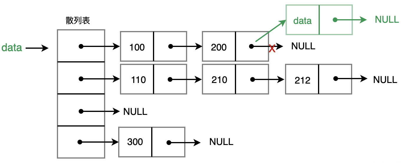
• Principle

  • The chaining method’score idea is to treat each array element as a bucket, and store multiple key-value pairs in the bucket.. Usually implemented using a linked list or an array.

  • Once a duplicate is found, insert the duplicate element intothe head or tail of the linked listthat’s it.

  • When querying, first find the corresponding position based on the hashed index value, thentake out the linked list, and query sequentially to find the desired data.

• Efficiency

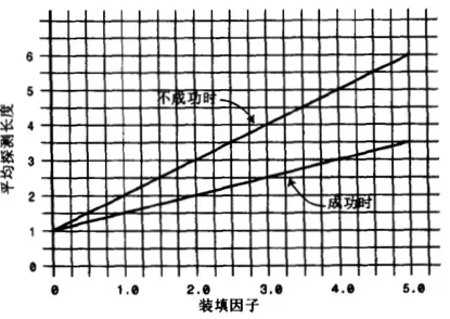
  • When implementing a hash table with chaining, the process of finding an element is divided into two parts:
    • Calculate the hash value and locate the slot: this step is a constant-time operation, usually 1 operation, independent of the length of the linked list.
    • Traverse the linked list to find the element: if multiple elements are in the same slot, the hash table searches the linked list of that slot. The average number of searches is half the length of the linked list, usually loadFactor / 2.
    • Therefore, a successful search may only need to look through half of the linked list: 1 + loadFactor/2. An unsuccessful search may need to query the entire linked list to know it failed: 1 + loadFactor.
  • The chaining method is relatively more efficient than the open addressing method, so in real development the chaining method is used more often. It does not cause a sharp performance drop after adding an element. For example, Java’s HashMap uses the chaining method.

Efficiency of the chaining method

Open addressing method

The open addressing method’sThe main working method is to find the next empty slot in the array to store the conflicting element when a hash collision occurs., there are three ways to probe empty slots:

• Linear probing

  • Linear probing (Linear Probing) is checking the next empty slot each time a collision occursindex = (hashFunc(key) + i) % tableSizewhere i is the number of collisions
  • Efficiency

  

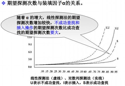
  Relationship between expected number of probes and load factor

  • Problem: Linear probing has a relatively serious problem, namely clustering.

    • For example, when there is no data and you insert 22-23-24-25-26, it means that the positions with indices 0-1-2-3-4 all have elements. This continuous filling of cells is called clustering.

    • Clustering affects the performance of the hash table, whether it is insertion, query, or deletion. For example, if we insert a 38, we will find that consecutive cells do not allow data to be placed, and in this process multiple probes are needed.

• Quadratic probing

  • Quadratic probing (Quadratic Probing) determines the position of the next slot based on the square of the number of collisionsindex = (hashFunc(key) + i^2) % tableSize
  • Optimizing the linear problem：
    • Linear probing can be viewed as probing with a step size of1, for example, starting from the index valuex, then linear probing isx+1，x+2，x+3sequential probing
    • Quadratic probing optimizes the step size., for example, from the index valuexstartx+1²，x+2²，x+3², so that a relatively long distance can be probed at one time, to avoid the impact caused by those clusters.
  • Efficiency：

  

  Performance of Quadratic Probing and Rehashing

  • problem：
    • Quadratic probing still has problems, for example, if consecutive insertions are32-112-82-2-192, then when accumulating in sequence, the step sizes are the same
    • That is, in this casewill cause a kind of clustering where the step sizes are all the same, which still affects efficiency.

• Rehashing

  • Rehashing (Double Hashing) uses a second hash function to calculate the step size and determine the position of the next slotindex = (hashFunc1(key) + i \* (constant - (hashFunc2(key) % constant))) % tableSize
  • Optimizing the quadratic probing problem:
    • The probe sequence step sizes generated by the quadratic probing algorithm are fixed: 1-4-9-16, and so on. Rehashing, on the other hand, applies another hash function to the key, performs hashing again, and uses the result of this hashing as the step size.
    • The second hashing must have the following characteristics:
      • It must be different from the first hash function (do not use the previous hash function again, otherwise the result will still be the original position)
      • It must not output 0 (otherwise there will be no step size, each probe will stay in place, and the algorithm will enter an infinite loop)
      • Computer experts have designed a hash function that works well:stepSize = constant - (hanshFunc(key) % constant), where constant is a prime number and is less than the capacity of the array.
  • Efficiency

  

  Performance of Quadratic Probing and Rehashing

Expansion/Shrinkage

• Expansion: As the amount of data increases, the bucket corresponding to each index becomes longer and longer, which causes a decrease in efficiency. Therefore, expand the array when appropriate, for example, double its size.

Expansion can simply double the capacity, but in this case all data items must be modified at the same time (re-call the hash function to obtain different positions). For example, a data item with hashCode = 12 is placed at index = 4 when arraySize = 8, and at index = 12 when arraySize = 16.

• ShrinkageWhen the load factor of the hash table (the ratio of the number of elements to the capacity of the hash table) falls below a certain threshold, shrinking is considered to save space and improve memory utilization efficiency.

When shrinking, the hash table capacity is usually reduced to half of its current capacity, and the positions of all existing elements are recalculated and reassigned.

When to expand/shrink?

A common case isloadFactor > 0.75when the load factor is greater than 0.75, expansion is performed. For example, Java’s hash table expands when the load factor exceeds 0.75.

Usually a lower load factor threshold is set, such as 0.25. When the load factor falls below this value, shrinking is triggered. However, excessive shrinking should also be avoided: a small, reasonable minimum capacity, such as 7 or 8, is usually set to ensure that the hash table maintains a certain capacity even when there are few elements, thereby avoiding frequent expansion and shrinking.

Hash Table Implementation

#include <stdio.h>
#include <string.h>

#define N 100003 // Hash table size (prime number, to reduce collisions)
#define M 200003 // Total number of nodes

// int to[M], key storage, stores the key of each node
// int val[M], value storage, stores the value of each node
// int head[N], bucket array (entry). head[5] = 3 means the linked list with hash value 5 starts at idx = 3.
// int nxt[M], linked list pointer (core), points to the index of the next node, equivalent to next in a linked list. nxt[3] = 7 means the next node of node 3 is 7.

int head[N], to[M], nxt[M], val[M];
int idx;

// Hash function
static int inline hash(int x)
{
        return (x % N + N) % N;
}

// Initialize
void hashtable_init()
{
        memset(head, -1, sizeof(head));
        idx = 0;
}

// Insert key -> value
void hashtable_put(int key, int value)
{
        int h = hash(key);
        to[idx] = key;
        val[idx] = value;
        nxt[idx] = head[h];
        head[h] = idx++;
}

// Look up key, return value (return -1 if not found)
int hashtable_get(int key)
{
        int h = hash(key);
        for (int i = head[h]; i != -1; i = nxt[i]) {
                if (to[i] == key)
                        return val[i];
        }
        return -1;
}

int main()
{
        hashtable_init();

        hashtable_put(1, 100);
        hashtable_put(2, 200);
        hashtable_put(100003, 300); // Test collisions

        printf("%d\n", hashtable_get(1)); // 100
        printf("%d\n", hashtable_get(2)); // 200
        printf("%d\n", hashtable_get(3)); // -1
}

Common algorithms

Hash

Problem	Links
P1 Two Sum✨✨✨	P1 Two Sum https://even629.com/posts/1/
P49 Group Anagrams	P49 Group Anagrams https://even629.com/posts/49/
P128 Longest Consecutive Sequence✨✨✨	P128 Longest Consecutive Sequence https://even629.com/posts/128/
P383 Ransom Note	P383 Ransom Note https://even629.com/posts/383/
P205 Isomorphic Strings	P205 Isomorphic Strings https://even629.com/posts/205/
P290 Word Pattern	P290 Word Pattern https://even629.com/posts/290/
P242 Valid Anagram	P242 Valid Anagram https://even629.com/posts/242/
P49 Group Anagrams	P49 Group Anagrams https://even629.com/posts/49/
P202 Happy Number	P202 Happy Number https://even629.com/posts/202/
P219 Contains Duplicate II✨✨✨	P219 Contains Duplicate II https://even629.com/posts/219/
P966 Vowel Spellchecker	P966 Vowel Spellchecker https://even629.com/posts/966/
P3484 Design Spreadsheet	P3484 Design Spreadsheet https://even629.com/posts/3484/
P380 Insert Delete GetRandom O(1)✨✨✨	P380 O(1) Time insertion、Delete and get random element https://even629.com/posts/380/
P3289 The Two Sneaky Numbers of Digitville	P3289 The Troublemaker in Digital Town https://even629.com/posts/3289/
P13 Roman to Integer	P13 Roman to Integer https://even629.com/posts/13/

Two pointers

Fast and slow pointers

Problem	Links
P234 Palindrome Linked List	P234 Palindrome Linked List https://even629.com/posts/234/
P142 Linked List Cycle II	P142 Linked List Cycle II https://even629.com/posts/142/
P80 Remove Duplicates from Sorted Array II ✨✨✨	P80 Remove Duplicates from Sorted Array II https://even629.com/posts/80/
P287 Find the Duplicate Number ✨✨✨	P287 Find the Duplicate Number https://even629.com/posts/287/
P19 Remove Nth Node From End of List	P19 Remove the Nth from the end of the linked list N node https://even629.com/posts/19/
P160 Intersection of Two Linked Lists	P160 Intersection of Two Linked Lists https://even629.com/posts/160/

Left and Right Pointers

Problem	Links
P283 Move Zeroes	P283 Move Zeroes https://even629.com/posts/283/
P125 Valid Palindrome	P125 Valid Palindrome https://even629.com/posts/125/
P27 Remove Element	P27 Remove Element https://even629.com/posts/27/
P167 Two Sum II - Input Array Is Sorted	P167 Two Sum II - Input sorted array https://even629.com/posts/167/
P88 Merge Sorted Array	P88 Merge Two Sorted Arrays https://even629.com/posts/88/
P392 Is Subsequence	P392 Is Subsequence https://even629.com/posts/392/
P75 Sort Colors	P75 Sort Colors https://even629.com/posts/75/
P31 Next Permutation	P31 Next Permutation https://even629.com/posts/31/
P15 3Sum ✨✨✨	P15 3Sum https://even629.com/posts/15/
P11 Container With Most Water ✨✨✨	P11 Container With Most Water https://even629.com/posts/11/
P611 Valid Triangle Number	P611 Number of valid triangles https://even629.com/posts/611/
P42 Trapping Rain Water ✨✨✨	P42 Trapping Rain Water https://even629.com/posts/42/

linked list

Problem	Links
P3217 Remove Nodes From Linked List Present in Array	P3217 Remove Nodes From Linked List Present in Array https://even629.com/posts/3217/
P141 Linked List Cycle	P141 Linked List Cycle https://even629.com/posts/141/
P2 Add Two Numbers	P2 Add Two Numbers https://even629.com/posts/2/
P21 Merge Two Sorted Lists	P21 Merge Two Sorted Linked Lists https://even629.com/posts/21/
P138 Copy List with Random Pointer	P138 Copy List with Random Pointer https://even629.com/posts/138/
P92 Reverse Linked List II	P92 Reverse Linked List II https://even629.com/posts/92/
P25 Reverse Nodes in k-Group ✨✨✨	P25 K Reverse Nodes in k-Group https://even629.com/posts/25/
P19 Remove Nth Node From End of List	P19 Remove the Nth from the end of the linked list N node https://even629.com/posts/19/
P82 Remove Duplicates from Sorted List II ✨✨✨	P82 Remove Duplicates from Sorted List II https://even629.com/posts/82/
P61 Rotate List	P61 Rotate List https://even629.com/posts/61/
P86 Partition List	P86 Partition List https://even629.com/posts/86/
P146 LRU Cache ✨✨✨	P146 LRUCache https://even629.com/posts/146/
P148 Sort List	P148 Sort List https://even629.com/posts/148/
P160 Intersection of Two Linked Lists	P160 Intersection of Two Linked Lists https://even629.com/posts/160/
P206 Reverse Linked List ✨✨✨	P206 Reverse Linked List https://even629.com/posts/206/
P234 Palindrome Linked List ✨✨✨	P234 Palindrome Linked List https://even629.com/posts/234/
P142 Linked List Cycle II ✨✨✨	P142 Linked List Cycle II https://even629.com/posts/142/
P24 Swap Nodes in Pairs	P24 Swap Nodes in Pairs https://even629.com/posts/24/

Tree

Binary Tree Traversal

Preorder (Depth-First), Inorder, Postorder, Level-order, Morris Traversal

Problem	Links
P104 Maximum Depth of Binary Tree	P104 Maximum Depth of Binary Tree https://even629.com/posts/104/
P100 Same Tree	P100 Same Tree https://even629.com/posts/100/
P226 Invert Binary Tree	P226 Invert Binary Tree https://even629.com/posts/226/
P101 Symmetric Tree	P101 Symmetric Binary Tree https://even629.com/posts/101/
P105 Construct Binary Tree from Preorder and Inorder Traversal✨✨✨	P105 Construct Binary Tree from Preorder and Inorder Traversal https://even629.com/posts/105/
P106 Construct Binary Tree from Inorder and Postorder Traversal✨✨✨	P106 Construct Binary Tree from Inorder and Postorder Traversal https://even629.com/posts/106/
P117 Populating Next Right Pointers in Each Node II	P117 Populating Next Right Pointers in Each Node II https://even629.com/posts/117/
P114 Flatten Binary Tree to Linked List✨✨✨	P114 Flatten Binary Tree to Linked List https://even629.com/posts/114/
P112 Path Sum	P112 Path Sum https://even629.com/posts/112/
P129 Sum Root to Leaf Numbers	P129 Sum Root to Leaf Numbers https://even629.com/posts/129/
P124 Binary Tree Maximum Path Sum✨✨✨	P124 Maximum Path Sum in Binary Tree https://even629.com/posts/124/
P173 Binary Search Tree Iterator	P173 Binary Search Tree Iterator https://even629.com/posts/173/
P222 Count Complete Tree Nodes✨✨✨	P222 Count Complete Tree Nodes https://even629.com/posts/222/
P236 Lowest Common Ancestor of a Binary Tree✨✨✨	P236 Lowest Common Ancestor of a Binary Tree https://even629.com/posts/236/
P199 Binary Tree Right Side View	P199 Binary Tree Right Side View https://even629.com/posts/199/
P637 Average of Levels in Binary Tree	P637 Average of Levels in Binary Tree https://even629.com/posts/637/
P102 Binary Tree Level Order Traversal	P102 Binary tree level order traversal https://even629.com/posts/102/
P103 Binary Tree Zigzag Level Order Traversal	P103 Binary Tree Zigzag Level Order Traversal https://even629.com/posts/103/
P530 Minimum Absolute Difference in BST	P530 Minimum Absolute Difference in BST https://even629.com/posts/530/
P98 Validate Binary Search Tree	P98 Validate Binary Search Tree https://even629.com/posts/98/
P230 Kth Smallest Element in a BST	P230 Kth in a Binary Search Tree K Smallest Element https://even629.com/posts/230/
P94 Binary Tree Inorder Traversal	P94 Binary Tree Inorder Traversal https://even629.com/posts/94/
P543 Diameter of Binary Tree✨✨✨	P543 Diameter of Binary Tree https://even629.com/posts/543/
P437 Path Sum III✨✨✨	P437 Path Sum III https://even629.com/posts/437/

Trie

A string as a node (C++ implementation)

struct TrieNode {
    std::string word;
    bool is_end;
    std::unordered_map<char, TrieNode *> children;
};

A char as a node

struct TrieNode {
    char data;
    bool is_end;
    std::unordered_map<char, TrieNode *> children;
};

// When char is limited to lowercase or uppercase letters, using vector is faster
struct TrieNode {
    char data;
    bool is_end;
    std::vector<TrieNode *> children;
};

Problem	Links
P14 Longest Common Prefix	P14 Longest Common Prefix https://even629.com/posts/14/
P208 Implement Trie (Prefix Tree)	P208 ImplementationTrie（Prefix tree） https://even629.com/posts/208/
P211 Add and Search Word - Data structure design	P211 Add and Search Word - Data Structure Design https://even629.com/posts/211/
P212 Word Search II✨✨✨	P212 Word Search II https://even629.com/posts/212/
P139 Word Break✨✨✨	P139 Word Break https://even629.com/posts/139/

Graph

DFS and BFS, Topological Sort

Problem	Links
P200 Number of Islands✨✨✨	P200 Number of Islands https://even629.com/posts/200/
P130 Surrounded Regions	P130 Surrounded Regions https://even629.com/posts/130/
P133 Clone Graph	P133 Clone Graph https://even629.com/posts/133/
P399 Evaluate Division	P399 Evaluate Division https://even629.com/posts/399/
P207 Course Schedule✨✨✨	P207 Course Schedule https://even629.com/posts/207/
P210 Course Schedule II✨✨✨	P210 Course Schedule II https://even629.com/posts/210/
P909 Snakes and Ladders✨✨✨	P909 Snakes and Ladders https://even629.com/posts/909/
P443 Minimum Genetic Mutation	P443 Minimum Genetic Change https://even629.com/posts/443/
P127 Word Ladder✨✨✨	P127 Word Ladder https://even629.com/posts/127/
P994 Rotting Oranges✨✨✨	P994 Rotting Oranges https://even629.com/posts/994/

Stack

Problem	Links
P20 Valid Parentheses	P20 Valid Parentheses https://even629.com/posts/20/
P71 Simplify Path	P71 Simplify Path https://even629.com/posts/71/
P155 Min Stack✨✨✨	P155 Min Stack https://even629.com/posts/155/
P150 Evaluate Reverse Polish Notation✨✨✨	P150 Evaluate Reverse Polish Notation https://even629.com/posts/150/
P224 Basic Calculator✨✨✨	P224 Basic Calculator https://even629.com/posts/224/
P394 Decode String✨✨✨	P394 Decode String https://even629.com/posts/394/
P2197 Replace Non-Coprime Numbers in Array✨✨✨	P2197 Replace non-coprime numbers in array https://even629.com/posts/2197/
P32 Longest Valid Parentheses✨✨✨	P32 Longest Valid Parentheses https://even629.com/posts/32/

Monotonic stack

Core rules of monotonic stackThat is:When pushing an element onto the stack, if it breaks monotonicity, pop the top until monotonicity is restored。

Suppose we want to maintain a ‘monotonically decreasing stack’ (smallest at the top)Either push, or pop several times and then push, always maintaining ‘monotonically decreasing’.

Type	In the stack, from bottom to top	Function
monotonically increasing stack	values are increasing	Suitable for finding the ‘next greater element’
Monotonically decreasing stack	values are decreasing	Suitable for finding the ‘next smaller element’

Its core idea is:

Use monotonicity to filter out useless elements, ensuring the ‘most recent valid element’ is at the top of the stack

Problem	Links
P3542 Minimum number of operations to make all elements 0 ✨✨✨	P3542 turn all elements into 0 the minimum number of operations https://even629.com/posts/3542/
P739 Daily Temperatures ✨✨✨	P739 Daily Temperatures https://even629.com/posts/739/
P84 Largest Rectangle in Histogram ✨✨✨	P84 Largest Rectangle in Histogram https://even629.com/posts/84/

Queue

Monotonic queue

Problem	Links
P239 Sliding Window Maximum	P239 Sliding Window Maximum https://even629.com/posts/239/

Matrix

Problem	Links
P73 Set Matrix Zeroes ✨✨✨	P73 Set Matrix Zeroes https://even629.com/posts/73/
P54 Spiral Matrix	P54 Spiral Matrix https://even629.com/posts/54/
P48 Rotate Image ✨✨✨	P48 Rotate Image https://even629.com/posts/48/
P240 Search a 2D Matrix II✨✨✨	P240 Search a 2D Matrix II https://even629.com/posts/240/
P36 Valid Sudoku	P36 Valid Sudoku https://even629.com/posts/36/
P289 Game of Life ✨✨✨	P289 Game of Life https://even629.com/posts/289/

Difference and Prefix Sum

2D difference and its prefix sum

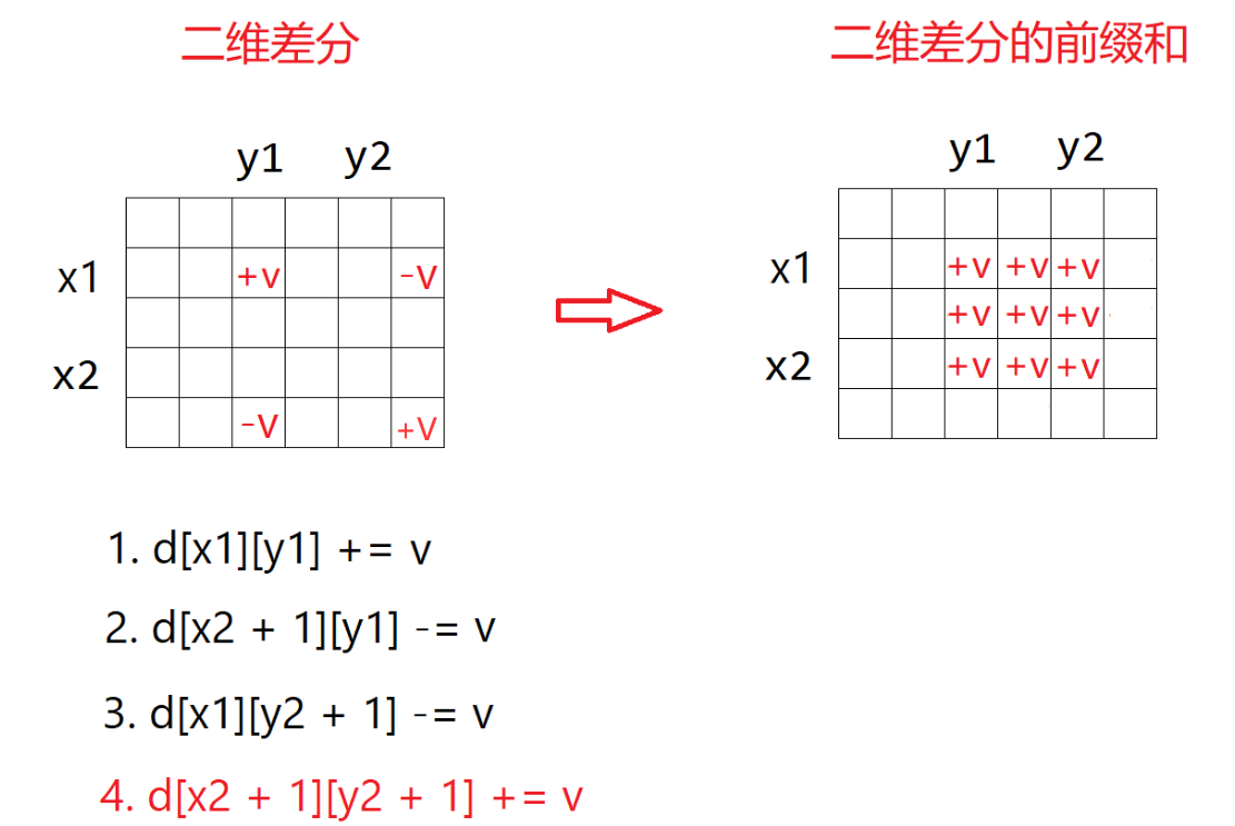
Problem	Links
P2536 Increment Submatrix Elements by One✨✨✨	P2536 Increment Submatrix Elements by One https://even629.com/posts/2536/

Sliding window

Classic Template

int left=0, right=0;
while(right < s.size()){
    windows.add(s[right]);
    right++;
    while(windows需要收缩){
        windows.remove(s[left]);
        left++;
    }
}

Problem	Links
P3 Longest Substring Without Repeating Characters	P3 Longest Substring Without Repeating Characters https://even629.com/posts/3/
P438 Find All Anagrams in a String	P438 Find All Anagrams in a String https://even629.com/posts/438/
P209 Minimum Size Subarray Sum	P209 Minimum Size Subarray Sum https://even629.com/posts/209/
P30 Substring with Concatenation of All Words ✨✨✨	P30 Substring with Concatenation of All Words https://even629.com/posts/30/
P76 Minimum Window Substring ✨✨✨	P76 Minimum Window Substring https://even629.com/posts/76/
P3186 Maximum Total Damage With Spell Casting	P3186 Maximum Total Damage of Spell Casting https://even629.com/posts/3186/

Backtracking

Solving a backtracking problem is essentially a traversal process of a decision tree.

Permutations of 1,2,3

You only need to think about three questions:

1. path: that is, the choices already made.
2. Choice list: that is, the choices you can currently make.
3. End condition: that is, the condition of reaching the bottom of the decision tree where no more choices can be made.

Classic template framework

result = []
void backtrace(路径，选择列表){
    if (满足结束条件){
        result.add(路径)
        return;
    }
    for(选择&: 选择列表){
        做选择，当前选择加入选择路径
        backtrace(路径, 选择列表)
        撤销选择，当前选择移除出选择路径
	}
}

Problem	Links
P46 Permutations	P46 Permutations https://even629.com/posts/46/
P78 Subsets	P78 subset https://even629.com/posts/78/
P17 Letter Combinations of a Phone Number	P17 Letter Combinations of a Phone Number https://even629.com/posts/17/
P39 Combination Sum	P39 Combination Sum https://even629.com/posts/39/
P22 Generate Parentheses✨✨✨	P22 Generate Parentheses https://even629.com/posts/22/
P79 Word Search	P79 Word Search https://even629.com/posts/79/
P212 Word Search II	P212 Word Search II https://even629.com/posts/212/
P51 N-Queens✨✨✨	P51 NQueen https://even629.com/posts/51/
P52 N-Queens II	P52 NQueen II https://even629.com/posts/52/
P77 Combinations	P77 Combination https://even629.com/posts/77/
P131 Palindrome Partitioning✨✨✨	P131 Palindrome Partitioning https://even629.com/posts/131/

Dynamic Programming

Problem	Links
P120 Triangle	P120 Triangle Minimum Path Sum https://even629.com/posts/120/
P1039 Minimum Score Triangulation of Polygon	P1039 Minimum Score of Polygon Triangulation https://even629.com/posts/1039/
P122 Best Time to Buy and Sell Stock II	P122 Best Time to Buy and Sell Stock II https://even629.com/posts/122/
P55 Jump Game	P55 Jump Game https://even629.com/posts/55/
P45 Jump Game II	P45 Jump GameII https://even629.com/posts/45/
P3147 Taking Maximum Energy From the Mystic Dungeon	P3147 Maximum Energy Drawn from a Mage https://even629.com/posts/3147/
P3186 Maximum Total Damage With Spell Casting	P3186 Maximum Total Damage of Spell Casting https://even629.com/posts/3186/
P3539 Sum of Array Products of Magic Sequences	P3539 Sum of array products of magic sequences https://even629.com/posts/3539/
P392 Is Subsequence	P392 Is Subsequence https://even629.com/posts/392/
P474 Ones and Zeroes	P474 Ones and Zeroes https://even629.com/posts/474/
P70 Climbing Stairs	P70 Climbing Stairs https://even629.com/posts/70/
P53 Maximum Subarray	P53 Maximum subarray sum https://even629.com/posts/53/
P918 Maximum Sum Circular Subarray	P918 Maximum Sum of Circular Subarray https://even629.com/posts/918/
P198 House Robber	P198 House Robber https://even629.com/posts/198/
P322 Coin Change	P322 Coin Change https://even629.com/posts/322/
P300 Longest Increasing Subsequence	P300 Longest Increasing Subsequence https://even629.com/posts/300/
P139 Word Break	P139 Word Break https://even629.com/posts/139/
P64 Minimum Path Sum	P64 Minimum Path Sum https://even629.com/posts/64/
P63 Unique Paths II	P63 Unique Paths II https://even629.com/posts/63/
P5 Longest Palindromic Substring	P5 Longest Palindromic Substring https://even629.com/posts/5/
P221 Maximal Square	P221 Maximal Square https://even629.com/posts/221/
P72 Edit Distance	P72 Edit Distance https://even629.com/posts/72/
P97 Interleaving String	P97 Interleaving String https://even629.com/posts/97/
P123 Best Time to Buy and Sell Stock III	P123 Best Time to Buy and Sell Stock III https://even629.com/posts/123/
P188 Best Time to Buy and Sell Stock IV	P188 Best Time to Buy and Sell Stock IV https://even629.com/posts/188/
P131 Palindrome Partitioning	P131 Palindrome Partitioning https://even629.com/posts/131/
P118 Pascal’s Triangle	P118 Pascal's Triangle https://even629.com/posts/118/
P279 Perfect Squares	P279 Perfect Squares https://even629.com/posts/279/
P152 Maximum Product Subarray	P152 Maximum Product Subarray https://even629.com/posts/152/
P416 Partition Equal Subset Sum	P416 Partition Equal Subset Sum https://even629.com/posts/416/
P32 Longest Valid Parentheses	P32 Longest Valid Parentheses https://even629.com/posts/32/
P62 Unique Paths	P62 Unique Paths https://even629.com/posts/62/
P1143 Longest Common Subsequence	P1143 Longest Common Subsequence https://even629.com/posts/1143/

Greedy

Problem	Links
P55 Jump Game✨✨✨	P55 Jump Game https://even629.com/posts/55/
P45 Jump Game II✨✨✨	P45 Jump GameII https://even629.com/posts/45/
P134 Gas Station✨✨✨	P134 Gas Station https://even629.com/posts/134/
P135 Candy✨✨✨	P135 Distribute Candy https://even629.com/posts/135/
P1578 Minimum Time to Make Rope Colorful	P1578 Minimum Time to Make Rope Colorful https://even629.com/posts/1578/
P3228 Maximum Number of Operations to Move Ones to the End	P3228 will 1 Maximum number of operations to move to the end https://even629.com/posts/3228/
P763 Partition Labels	P763 Partition Labels https://even629.com/posts/763/
P121 Best Time to Buy and Sell Stock	P121 Best Time to Buy and Sell Stock https://even629.com/posts/121/
P976 Largest Perimeter Triangle	P976 Maximum Perimeter of a Triangle https://even629.com/posts/976/

Sort

Merge Sort, Counting Sort, Quick Sort, Heap Sort

Problem	Links
P148 Sort List	P148 Sort List https://even629.com/posts/148/
P2785 Sort Vowels in a String	P2785 Sort the vowels in a string https://even629.com/posts/2785/
P3541 Find the Vowel and Consonant with the Highest Frequency	P3541 Find the most frequent vowel and consonant https://even629.com/posts/3541/
P274 H-Index	P274 Hindex https://even629.com/posts/274/
P3005 Count Elements With Maximum Frequency	P3005 Count Elements With Maximum Frequency https://even629.com/posts/3005/

Quicksort

Lomuto partition

Each partition determines the position of one value.

#include <vector>
#include <algorithm>
using std::vector;

int partition(vector<int> &arr, int start, int end)
{ // Partition interval [l, r]
        int pivot = arr[end];
        int i = start; // Right boundary of the region less than pivot

        for (int j = start; j < end; j++) {
                if (arr[j] < pivot) { // Put elements less than pivot on the left
                        std::swap(arr[i], arr[j]);
                        i++;
                }
        }
        std::swap(arr[i], arr[end]); // Place pivot in its correct position
        return i; // Return the final position of pivot
}

void quick_sort(vector<int> &arr, int start, int end)
{
        if (start >= end)
                return;
        int p = partition(arr, start, end);
        quick_sort(arr, start, p - 1);
        quick_sort(arr, p + 1, end);
}

#include <stdio.h>
int main()
{
        vector<int> arr = { 1, 3, 6, 2, 3, 8, 4, 9, 0 };
        quick_sort(arr, 0, arr.size() - 1);
        for(int num: arr){
                printf("%d ", num);
        }
        printf("\n");
}

Hoare partition

It does not require pivot to end up in the correct position, but guarantees:

• $[start .. left-1] < pivot$
• $[left .. end] >= pivot$

#include <vector>
using std::vector;


// 4、5、8、1、7、2、6、3 // pivot = 4, left = arr[0]=4 right=arr[n-1] =3

// 3, 5, 8, 1, 7, 2, 6, 4 // left->5  right->6

// 3, 2, 8, 1, 7, 5, 6, 4 // left->8  right->7

// 3, 2, 1, 8, 7, 5, 6, 4 // left->1 right->8  right<left, stop

/*
* Hoare partition the normal logic of，It does not require pivot to end up in the correct position，but guarantees：
* [start .. left-1] < pivot
* [left .. end] >= pivot
 */

int partition(vector<int> &arr, int start, int end)
{
        int pivot = arr[start];
        int left = start, right = end;

        while (left <= right) {
                while (arr[left] < pivot) {
                        left++;
                }
                while (arr[right] > pivot) {
                        right--;
                }
                if (left <= right) {
                        std::swap(arr[left], arr[right]);
                        left++;
                        right--;
                }
        }
        return left;
}

void quick_sort(vector<int> &arr, int start, int end)
{
        if (start >= end) {
                return;
        }
        int p;
        p = partition(arr, start, end);
        quick_sort(arr, start, p - 1);
        quick_sort(arr, p, end);
}

#include <stdio.h>
int main()
{
        vector<int> arr = { 1, 3, 6, 2, 3, 8, 4, 9, 0 };
        quick_sort(arr, 0, arr.size() - 1);
        for(int num: arr){
                printf("%d ", num);
        }
        printf("\n");
}

It can also be written this way (recommended approach)

// Quick sort function (Hoare partition scheme implementation)
void quickSort(vector<int>& nums, int l, int r) {
    // 1. Recursion termination condition: when the subarray length is 1 or empty, no sorting is needed
    if (l >= r) return;

    // 2. Initialize partition parameters:
    // - i initially to the left of the left boundary (l-1)
    // - j initially to the right of the right boundary (r+1)
    // - Choose the middle element as the pivot x (to avoid worst-case time complexity in extreme cases such as fully sorted arrays)
    int i = l - 1, j = r + 1;
    int x = nums[(l + r) >> 1]; // Use bitwise operation instead of (l + r) / 2, equivalent and more efficient

    // 3. Hoare partition loop: two pointers move from both ends toward the middle
    while (i < j) {
        // 3.1 Move left pointer i: skip all elements less than x until finding an element >= x
        do i++; while (nums[i] < x);

        // 3.2 Move right pointer j: skip all elements greater than x until finding an element <= x
        do j--; while (nums[j] > x);

        // 3.3 If the pointers have not crossed, swap the elements at the left and right pointers (ensuring left <= x and right >= x)
        if (i < j) swap(nums[i], nums[j]);
    }

    // 4. Recursively sort the left and right subarrays:
    // - The partition point is j (because when i >= j, j is the rightmost end of the left half)
    // - Left subarray: [l, j] (all elements <= x)
    // - Right subarray: [j+1, r] (all elements >= x)
    quickSort(nums, l, j);
    quickSort(nums, j + 1, r);
}

Reference Problems

Problem	Links
P215 Kth Largest Element in an Array	P215 The kth in the arrayKlargest element https://even629.com/posts/215

Heap sort

forComplete binary treeNumber the nodes, and the following relationships hold

Item	1-based numbering(root=1)	0-based numbering(root=0)
Left child	$\text{left}(i)=2i$	$\text{left}(i)=2i+1$
Right child	$\text{right}(i)=2i+1$	$\text{right}(i)=2i+2$
Parent node	$\text{parent}(i)=\lfloor i/2 \rfloor（i>1）$	$\text{parent}(i)=\lfloor (i-1)/2 \rfloor（i>0）$
Condition for having at least a left child	$2i \le n$	$2i+1 < n$
Condition for right child existence	$2i+1 \le n$	$2i+2 < n$
Leaf node condition	$i > \lfloor n/2 \rfloor$	$i > \lfloor (n-2)/2 \rfloor$ or $2i+1 \ge n$
Condition for having only a left child	$2i = n$	$2i+1 < n$ and $2i+2 \ge n$
Depth (root level=1)	$\lfloor \log_2 i \rfloor +1$	$\lfloor \log_2 (i+1) \rfloor +1$
Depth (root level=0)	$\lfloor \log_2 i \rfloor$	$\lfloor \log_2 (i+1) \rfloor$

#include <vector>
using std::vector;

void heapify(vector<int> &vec, int curr, int n)
{
        int left = curr * 2 + 1;
        int right = curr * 2 + 2;
        int largest = curr;

        if (left < n && vec[left] > vec[largest]) {
                largest = left;
        }

        if (right < n && vec[right] > vec[largest]) {
                largest = right;
        }

        if (largest != curr) {
                std::swap(vec[largest], vec[curr]);
                //Since the parent and child nodes are swapped, the child's subtree may be affected, so adjust the child's subtree.
                heapify(vec, largest, n);
        }
}

void buildMaxHeap(vector<int> &vec)
{
        int n = vec.size();
        // The last node is at position n-1, so its parent is at (n-1-1)/2.
        for (int i = (n - 2) / 2; i >= 0; i--) {
                heapify(vec, i, n);
        }
}

#include <stdio.h>

int main()
{
        vector<int> nums = { 9, 8, 2, 1, 5, 3, 0, 10, 22, 5 };
        int n = nums.size();
        buildMaxHeap(nums);

        for (int i = 0; i < n; i++) {
                // pop
                std::swap(nums[0], nums[n - i - 1]);
                heapify(nums, 0, n - i - 1); // Heap length is n-i-1
        }
        // Output the sorted array
        for (int i = 0; i < n; i++)
                printf("%d ", nums[i]);
        printf("\n");
}

Problem	Links
P3408 Design Task Manager	P3408 Design Task Manager https://even629.com/posts/3408/
P407 Trapping Rain Water II✨✨✨	P407 Trapping Rain WaterII https://even629.com/posts/407/
P215 Kth Largest Element in an Array	P215 The kth in the arrayKlargest element https://even629.com/posts/215/
P373 Find K Pairs with Smallest Sums	P373 Find the smallest sumKpairs of numbers https://even629.com/posts/373/
P295 Find Median from Data Stream✨✨✨	P295 Median of Data Stream https://even629.com/posts/295/
P239 Sliding Window Maximum	P239 Sliding Window Maximum https://even629.com/posts/239/
P347 Top K Frequent Elements	P347 top K frequent elements https://even629.com/posts/347/
P502 IPO	P502 IPO https://even629.com/posts/502/

Divide and Conquer

The essence of binary search is:Finding the position of the first element in a sequence that satisfies a certain condition。

The confusing part of binary search is usually: when to use <= in the while loop and when not to use the equals sign;

First consider elements sorted in ascending order (descending is equivalent), and it should be divided into two cases:

1. No duplicate elements;

The problem in this case is generally: find whether a target element appears in the sequence; if it appears, return its index; if it does not appear, return the position where it should be inserted.

That is, determine an interval [x, x], where target is the element at position x. If this element does not exist, then the determined interval is [x+1, x], with the left boundary greater than the right boundary, meaning there is no element in the interval.

#include <vector>
using std::vector;

class Solution {
    public:
        int searchInsert(vector<int> &nums, int target)
        {
                int n = nums.size();
                int left = 0, right = n - 1, mid = 0;

                while (left <= right) {
                        mid = left + (right - left) / 2;

                        if (nums[mid] < target)
                                left = mid + 1;
                        else if (nums[mid] > target)
                                right = mid - 1;
                        else
                                return mid;
                }
                

                return left;
        }
};

2. There are duplicate elements. The latter is a generalization of the former, meaning the latter’s algorithm also applies to the former.

The problem in this case is to determine two subproblems: the index of the first element greater than or equal to target, and the index of the first element greater than target.

(1) Find the lower bound (the index of the first element greater than or equal to target, the x in [x, y))

int LowerBound(const std::vector<int>& a, int target)
{
    int left = 0, right = a.size(), mid;
    while (left < right) {
        mid = left + (right - left) / 2;
        if (a[mid] >= target) {
            // If the middle number is greater than or equal to target, search in the left subinterval [left, mid]
            right = mid;
        } else {
            // If the middle number is less than target, search in the right subinterval [mid+1, right]
            left = mid + 1;
        }
    }
    // If left == right, returning either one is fine.
    return left;
}

(2) Find the upper bound (the index of the first element greater than target, the y in [x, y))

int UpperBound(const std::vector<int>& a, int target)
{
    int left = 0, right = a.size(), mid;
    while (left < right) {
        mid = left + (right - left) / 2;
        if (a[mid] > target) {
            // If the middle number is greater than target, search in the left subinterval [left, mid]
            right = mid;
        } else {
            // If the middle number is less than or equal to target, search in the right subinterval [mid+1, right]
            left = mid + 1;
        }
    }
    // If left == right, returning either one is fine.
    return left;
}

Take the following problem as an example:

P34 Find First and Last Position of Element in Sorted Array

https://even629.com/posts/34

#include <vector>

using std::vector;

class Solution {
    private:
        int search_range_end(vector<int> &nums, int target)
        {
                int n = nums.size();
                int left = 0, right = n - 1, mid;
                while (left < right) {
                        mid = left + (right - left + 1) / 2;
                        if (nums[mid] <= target)
                                left = mid;
                        else
                                right = mid - 1;
                }

                return (nums[left] == target) ? left : -1;
        }
        int search_range_start(vector<int> &nums, int target)
        {
                int n = nums.size();
                int left = 0, right = n - 1, mid;
                while (left < right) {
                        mid = left + (right - left) / 2;
                        if (nums[mid] >= target)
                                right = mid;
                        else
                                left = mid + 1;
                }

                return (nums[left] == target) ? left : -1;
        }

    public:
        vector<int> searchRange(vector<int> &nums, int target)
        {
                if (nums.empty())
                        return { -1, -1 };

                vector<int> res(2);
                res[0] = search_range_start(nums, target);
                res[1] = search_range_end(nums, target);
                return res;
        }
};

When finding end, you need to use the upper median (upper mid):mid = left + (right - left + 1) / 2;This ensures mid > left, so the interval is guaranteed to shrink.

Problem	Links
P34 Find First and Last Position of Element in Sorted Array✨✨✨	P34 Find First and Last Position of Element in Sorted Array https://even629.com/posts/34/
P108 Convert Sorted Array to Binary Search Tree	P108 Convert Sorted Array to Binary Search Tree https://even629.com/posts/108/
P148 Sort List	P148 Sort List https://even629.com/posts/148/
P427 Construct Quad Tree	P427 Construct Quad Tree https://even629.com/posts/427/
P23 Merge k Sorted Lists	P23 MergeKsorted linked lists https://even629.com/posts/23/
P35 Search Insert Position	P35 Search Insert Position https://even629.com/posts/35/
P74 Search a 2D Matrix	P74 Search a 2D Matrix https://even629.com/posts/74/
P240 Search a 2D Matrix II✨✨✨	P240 Search a 2D Matrix II https://even629.com/posts/240/
P162 Find Peak Element	P162 Find Peak Element https://even629.com/posts/162/
P33 Search in Rotated Sorted Array	P33 Search in Rotated Sorted Array https://even629.com/posts/33/
P153 Find Minimum in Rotated Sorted Array	P153 Find Minimum in Rotated Sorted Array https://even629.com/posts/153/
P4 Median of Two Sorted Arrays	P4 Find the Median of Two Sorted Arrays https://even629.com/posts/4/

Disjoint Set Union (DSU)

Problem	Links
P3607 Power Grid Maintenance	P3607 Power Grid Maintenance https://even629.com/posts/3607